Topographie des planètes - Master 2 - Parcours Planétologie Ile de France Cours 1 - Parcours Planétologie Ile de France
←
→
Transcription du contenu de la page
Si votre navigateur ne rend pas la page correctement, lisez s'il vous plaît le contenu de la page ci-dessous
Master 2 - Parcours Planétologie Ile de France
               http://planeto.geol.u-psud.fr/master

                          Cours 1

       Topographie des
          planètes
   Frédéric Schmidt - frederic.schmidt@u-psud.fr
          http://planeto.geol.u-psud.fr/Frederic-Schmidt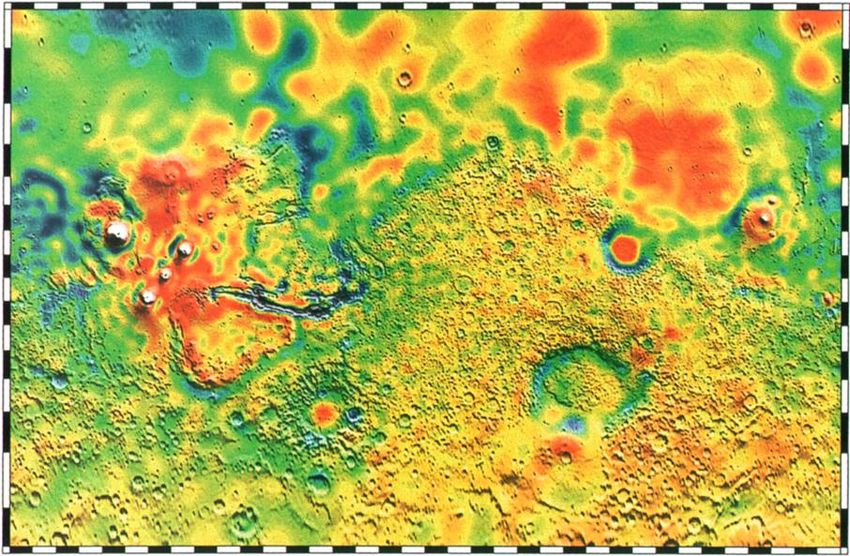
Plan

• Définitions
• Mesure de la topographie
 • Principe, incertitudes
• Quelles interprétations planétologiques ?
Plan

• Définitions
• Mesure de la topographie
 • Principe, incertitudes
• Quelles interprétations planétologiques ?
Forme théorique
                    d’une planète
Clairaut (XVIIIème siècle)

               • Equilibre
                  hydrostatique d’une
                  sphère en rotation
                  • forme
                  • rotation
                  • inertie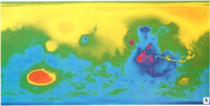
Géoïde               Terre

Forme d’une planète ?
•   Surface de potentiel de référence

    •   force de gravité

    •   force centrifuge
                                                Mars
•   Description :

    •   variation du rayon à chaque point

    •   variation de gravité à rayon constant
        (ou sur une ellipsoïde)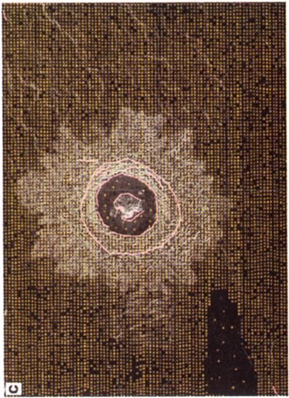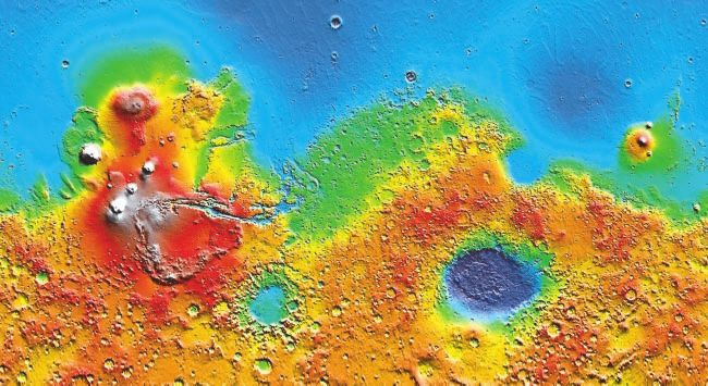
Géoïde terrestre
Définition :
• surface moyenne des
   océans (interface entre
   deux fluides à l’équilibre
   hydrostatique)

                                     représentation avec
                                exagération verticale x 10 000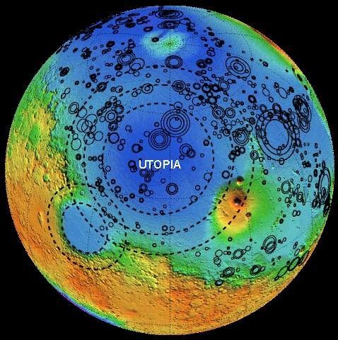
Géoïde terrestre
Définition :
• surface moyenne des
   océans (interface entre
   deux fluides à l’équilibre
   hydrostatique)

                                     représentation avec
                                exagération verticale x 10 000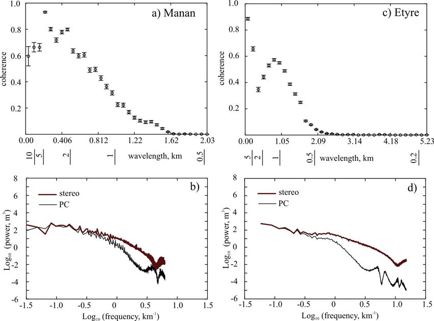
Géoïde Martien : Areoïde
Définition :
• Ancienne : surface de 6.1
       Mbar (proche du point
       triple de l’eau) MAIS
       variation temporelle !
• MOLA : surface de
                                                                                                     LEMOINE ET AL.: AN IMPROVED MARS GRAVITY MODEL               23,

                                                                                                       0ø                                       0ø

       potentiel équatorial moyen
       (rayon 3396 km)
  Smith, D. E. & Zuber, M. T., The relationship between MOLA northern hemisphere
  topography and the 6.1-Mbar atmospheric pressure surface of Mars, Geophys. Res. Lett.,
  AGU, 1998, 25, 4397-4400
  Lemoine, F. G.; Smith, D. E.; Rowlands, D. D.; Zuber, M. T.; Neumann, G. A.; Chinn, D. S.
  & Pavlis, D. E., An improved solution of the gravity field of Mars (GMM-2B) from Mars
  Global Surveyor, J. Geophys. Res., AGU, 2001, 106, 23359-23376                                                                                        I• mGal
                                                                                              -5OO                 0                5OO               IOO0

                                                                                                              GMM-2B to degree 60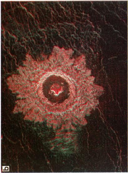
Ellipse de référence /
Datum / Système géodésique
 Ellipse ajustant la forme (géoïde) à l’échelle globale/locale
Altitude

ATTENTION
plusieurs
définition !?

H : altitude

                           http://www.geod.nrcan.gc.ca/hm/images/fig1_heights_f.jpg
Représentation cartographique Coordonnées ? Projection sur un plan
Harmoniques sphériques

 • Projection des données dans une nouvelle
   base (orthogonale, normée)
 • Equivalent à la Transformé de Fourier :
   spatiale, sphérique
Harmoniques sphériques

   • Degré 1

   • Degré 2

   • Degré 36
   • ...
Filtrage par harmonique
        sphérique
 • Reconstruction de la topographie terrestre
Degré 1         Degré 1 à 6       Degré 1 à 36
Plan • Définitions • Mesure de la topographie • Principe, incertitudes • Quelles interprétations planétologiques ?
Mesure de topographie
Comment calculer l’altitude ?
Mesure de topographie
    Comment calculer l’altitude ?
•   Mesure du champs de gravité par des gravimètres
    (création du géoïde)
• Mesure de la topographie (forme de la planète)
• Ajustement de l’ellipsoïde de référence (nécessaire
    pour la cartographie)
• Calcul de l’altitude et de la coordonnée
    géographique
Mesure de topographie Comment calculer l’altitude ? • Mesure du géoïde par des gravimètres • Mesure de la topographie (forme de la planète) • Ajustement de l’ellipsoïde de référence • Calcul de l’altitude
Mesure de topographie
• Trajet aller-retour d’une onde :
 • radar, laser
• Stéréographie
 • imagerie visible, radar
• Photoclinométrie
 • imagerie visible
• Limitations ? Incertitude ?
Exemple d’instruments
• •LaserMars : MOLA (Mars Global Surveyor, 1999)
    •   Lune : LOLA (Lunar Reconnaissance Orbiter, 2009)
    •   Mercure : MLA (Messenger, 2011), BELA (Bepi Columbo, 2020 ?)

•    Radar
    • Venus : radar experiment (Pioneer Venus, 1980), SAR (Magellan, 1990)
    • Mars : MARSIS (Mars Express, 2003), SHARAD (Mars Reconnaissace Orbiter, 2005)
    • Satellites saturniens (Titan, Encelade,...) : RADAR (Cassini, 2004)
•    Stéréographie
    • Mars : HiRISE (Mars Reconnaissace Orbiter, 2005)
    • Mars : HRSC (Mars Express, 2004)
    • Satellites galiléens: PhotoPolarimeter/Radiometer (Galileo, 1995)
•    Photoclinométrie
    • Mars : HiRISE (Mars Reconnaissace Orbiter, 2005)
    • Satellites galiléens: PhotoPolarimeter/Radiometer (Galileo, 1995)
Principe : aller-retour • Mesure du temps d’aller retour : t Détecteur • Vitesse de propagation connu : v • Positionnement du satellite connu • distance : d=v.t/2 • Laser et Radar • visée Nadir surface
Principe : aller-retour
• Mesure du temps d’aller retour : t   Détecteur

• Vitesse de propagation connu : v
• Positionnement du satellite connu
• distance : d=v.t/2
• Laser et Radar
• visée Nadir                            surface
Zuber et al. (1992) and Abshire et al. (2000). We advise the                    filt
                 reader to refer to these two sources for more detail.                           tio
                    The MOLA laser operates at a wavelength of 1.064 µm. Pulses

        Principe : aller-retour
                                                                                                 ma
                 are emitted with a repetition rate of 10 Hz. A ranging schematic                (Ta
                 is shown in Fig. 1. The basic properties of the laser and the                   op
                                                                                                 of
                                                                                                 gre
                                                                                                 If
Mesure :
• temps
d’aller-retour
• dispersion
de l’onde
• Idem radar                                                                                     De
et laser                                                                                         Ch
                                                                                                 Te

                    FIG. 1. Laser ranging schematic. Range to the surface R = c!T /2; !T =       Fo
                 Tr − T0 ; T0 —transmitted pulse time; Tr —received time; E 0 —transmitted en-   Pro
                 ergy; Er —received energy. Detector can only register incoming photons when
                 the range gate is open.                                                           a
Perturbations Laser
198 IVANOV AND MUHLEMAN
• Incertitude de
position du
satellite
• Présence de
nuage
FIG. 7. Samples of cloud formations for the south polar region. Horizontal scale is equal to 2050 km. Vertical exaggeration is about 1:50. These four graphs
illustrate the most extensive cloud formations encountered during the first south winter. Channel 1 returns are marked with black crosses; channel 4 returns are
marked with blue diamonds. Clusters of channel 1 clouds in the latitude band from 80◦ S to 70◦ S are evident in orbits 1640, 1654, 10075. Clouds located over the
pole are similar to the North polar cloud formations in Fig. 5. In orbit 1640, a channel 4 cloud formation is observed inside a channel 1 formation.
composed of CO2 ice, but weIvanov, A. B. & Muhleman, D. O., Cloud Reflection Observations: Results from
can’t rule out water ice as one of Most of the cloud echoes are detected during the polar night.
the Mars Orbiter Laser Altimeter, Icarus, 2001, 154, 190-206
the possible components. We think that we observe nighttime clouds only, because the tem-
perature drops low enough to permit condensation of detectable
clouds. Background radiation from Mars would not preclude
3.4. North and South Comparison and Analysis
MOLA from seeing clouds, should there be any (such as aphe-
In the following section we summarize and compare our lion water ice clouds, that greatly attenuate MOLA’s receivedForma- tends from "220°E to "300°E and from curves northeastward in a “scorpion tail” pat-
Downloaded from www.sciencemag.org on Nove
Borealis "50°S to "20°N and spans about 107 km2 in tern. This arcuate ridge bounds Solis Planum,
d small area. The highest portion of the southern rise a plateau within the southern rise. The ridge
Exemple : Mars (MOLA)
mentary contains the Tharsis Montes (Ascraeus, Pavo- contains an abundance of heavily cratered
r these nis, and Arsia). Eastward of the highest ter- Noachian material that has presumably es-
achian- rain but still elevated are the ridged plains of caped resurfacing by younger Tharsis volca-
flat in- Lunae Planum (Fig. 2). The smaller northern nic flows because of its high elevation. It has
Hespe- rise is superposed on the lowlands and covers been suggested (25) that the termination of
Précision :
• verticale : 1m
• horizontale :
300m
Smith, D. E.; Zuber, M. T.; Solomon, S. C.; Phillips, R. J.; Head, J.
W.; Garvin, J. B.; Banerdt, W. B.; Muhleman, D. O.; Pettengill, G. H.;
Neumann, G. A.; Lemoine, F. G.; Abshire, J. B.; Aharonson, O.;
Brown, D. C.; Hauck, S. A.; Ivanov, A. B.; McGovern, P. J.; Zwally,
H. J. & Duxbury, T. C., The Global Topography of Mars and
Implications for Surface Evolution, Science, 1999, 284, 1495-+
28 MAY 1999 VOL 284 SCIENCE www.sciencemag.orgas the transmitter frequency exceeds the local plasma fre-
nd By sequentially stepping the transmitter frequency after directly. However, the plasma frequency can be determined
ns eachquency, electromagnetic
transmit-receive cycle, thewave
timepropagation can the
delay, and hence start to
from the harmonic spacing and is fp(local) = 0.09 MHz. At
Perturbations Radar
an occur.
range Remote
to the echoes
reflection point,from
can bethedetermined
ionosphere as can then be
a func- somewhat higher frequencies a very strong ionospheric
to tiondetected, starting
of frequency. initially
A plot of theattime
zerodelay
time asdelay, and then
a function of with echo trace can be seen extending from about 0.6 to
gs a steadily
frequency, increasing
Dt(f), can thentime
be delay
made,asasthe range tointhe
illustrated thereflec- 2 MHz, with time delays ranging from about 2.5 to
nts tion point increases. These echoes produce the trace labeled
3.5 ms. The echo trace ends in a well-defined cusp at
nd ‘‘ionospheric echo’’ in Fig. 1. As the transmitter frequency
les approaches the maximum plasma frequency in the iono-
sphere, fp(max), the time delay increases rapidly, forming
an the left-hand branch of the feature labeled ‘‘cusp’’. The
he cusp occurs because the group velocity goes to zero over
n- a rapidly increasing path length as the frequency
n- approaches fp(max). As soon as the transmitter frequency
he exceeds fp(max) the pulse can pass through the ionosphere
of to the surface of the planet, where it reflects and returns to
þ
. the spacecraft, forming the right-hand branch of the cusp.
so By measuring the time delay as a function of frequency,
les the function Dt(f) on the left-hand side of Eq. (1) can be
res determined. To obtain the electron density as a function
as,
of altitude, the problem is then to solve for the function
nd
fp(z) inside the integral. The solution of this integral equa-
els
tion, called Abel’s equation, is a classical problem in math-
he
mic
ematical physics (Whittaker and Watson, 1927), and has a
nd formal solution (Budden, 1961) given by
of Z
2 p=2
de zðfp Þ ¼ cDtðfp sin aÞda; ð2Þ
p a0
ars Fig. 2. A color-coded ionogram showing the echo intensity as a function
re- where sin a = fp(z)/f and sin a0 = fp(zsc)/fp(max). Since time of the time delay, Dt, and frequency, f. To provide a rough estimate of the
aft range to the reflection point, the scale on the right gives the apparent
delay measurements must be made at a discrete set of fre- range, which is defined as cDt/2, where c is the speed of light. The white
ag- quencies, to apply this equation the integral must be line shows the time delay computed from Eq. (1) using the dispersion-
mes
Fig.converted to shows
1. The top panel a discrete sum ofprofile
a representative integrals. The integration
of the electron plasma corrected plasma frequency profile shown in Fig. 3.
will
frequency, fp, in the Martian ionosphere, and the bottom panel shows the
in corresponding ionogram, which is a plot of the time delay, Dt, for a
an sounder pulse of frequency, f, to reflect from the ionosphere and return to Gurnett, D.; Huff, R.; Morgan, D.; Persoon, A.; Averkamp, T.; Kirchner, D.; Duru, F.;
the spacecraft. Akalin, F.; Kopf, A.; Nielsen, E.; Safaeinili, A.; Plaut, J. & Picardi, G., An overview of
radar soundings of the martian ionosphere from the Mars Express spacecraft, Advances
in Space Research, 2008, 41, 1335-13465.6 Angle d'incidence
Perturbations : réflectance
L'angle d'incidence décrit la relation entre l'illumination du radar et la surface d
Plus concrètement, c'est l'angle entre le faisceau du radar et l'objet ciblé. L'angle
d'incidence détermine l'apparence de la cible sur une image.
Un angle d'incidence local peut être déterminé pour chaque pixel d'une image. L
surfaces retournant un signal fort et qui sont brillantes sur l'image radar peuvent retourner présense d'arbres, rochers, édifices et autres structures font varier l'angle d'incide
un signal faible dans la portion du visible et de l'infrarouge du spectre électromagnétique local. Ceci génère des variations de l'intensité du pixel.
et apparaître sombre sur une photographie, une image de Landsat ou de SPOT.
Rétro-diffusion de l’énergie dépends de :
Rugosité de surface
La rugosité de surface influe sur la réflectivité du rayonnement des hyperfréquences.
Les surfaces lisses et horizontales, qui réfléchissent presque toute l'énergie incidente en
• angle d’incidence
direction opposée au radar, sont appelées réflecteurs spéculaires. Ces surfaces, comme
l'eau calme ou les routes pavées, apparaissent foncées sur les images radar.
• rugosité
• matériaux (constantes diélectrique)
variations de l'intensité du pixel
Les angles d'incidence des satellites varient moins que les angles d'incidence de
A formes
= antenne; h = variations
aéroportées, de hauteur
car leur deest
altitude beaucoup =plus
la surface; longueur d'onde
élevée. Cecidu radar.une
donne
Surface de rugosité intermédiaire; réflecteur moyen; retour d'une petite partie du
illumination plus uniforme sur les images spatiales que sur les images aériennes. signal.
rugosité de surface influe sur la réflectivité
A = antenne; h = variations de hauteur de la surface; = longueur d'onde du radar.
Surface lisse; réflecteur presque parfait (spéculaire); pas de retour de signal.
A = antenne; h = variations de hauteur de la surface; = longueur d'ondehdu= radar.
A = antenne; variations de hauteur de la surface; = longueur d'onde du radar.
Surface de rugosité intermédiaire; réflecteur moyen; retour d'une
Surface departie
petite du importante;
rugosité signal. réflecteur diffus; retour d'une grande partie du signal.
La rugosité de surface est fonction de la longueur d'onde et de l'angle d'incidence duIces, Oceans, and Fire: Satellites of the Outer Solar System (2007)
Radargramme Titan
occasional relief of >500 m. Perhaps, as shown in
Figs. 1 and 2, the most intriguing feature of the altime-
ter echoes is the wide range of “depths” seen.
R
Scien
441.
fan,
2007
• RADAR - Cassini
312
A
the J
• Diamètre de Tech
Titan : 2575 km
• Résolution au sol
entre 60 km et 25
km
Figure 1: Radargram of T19 altimetry : Red repre-
sents strongest signal while the width is related to the
surface properties such as material and slope. The
spacecraft altitude varies from about 4000 km on the
left to 10,000 on the right.Sources d’incertitudes :
aller/retour
• Incertitude de géométrie (position du
satellite, direction de visée)
• Perturbation de l’onde (nuages, ionosphère,...)
• Réflexion en surface (topographie, matériaux)Principe : stéréoscopie • Paire d’image • Points d’appui commun • Parallaxe
Principe : stéréoscopie

Parallaxe : Pa = xa - xa'
Parallaxe : P = xPP2’ - xPP1=xPP2 - xPP1’
Distance entre les points Nadir: B
Altitude du détecteur : H
Distance focale de la lentille : f

Hauteur en A : ha = H - (B.f)/Pa
∆hab=H.(Pa-Pb)/(P+Pa-Pb)
Exemple
                 Tête de Mars observé par MOC

     Paire
stéréoscopique

  Anaglyphe                  Modèle 3d
Exemple
• HRSC, Mars Express
• résolution altitude relative < 300 m
9 canaux
Promethei Terra, hourglass cratersIncertitude : stéréoscopie • Densité de point d’appui (forme du terrain) • Incertitude de géométrie • Perturbation de l’onde (nuages,...)
1941ApJ....93..403M
       Principe : photoclinométrie

•   Shape-from-shading

•   Hypothèses:
    milieux homogène
    réflectance connu

                                                                                                     pA
•   Energie en O :                                                                         iA
    Trajet LAO : EA=L.cos(iA).R(LA,AO)
    Trajet LBO : EB=L.cos(iB). R(LB,BO)
                                                                                                      φA         i
    φA ≃ φB
    pA= i+ iA
    pB= i+ iB
                                                                                                   iB φ B
                                                                                                            pB
                  M. Minnaert, The reciprocity Principle in Lunar Photometry , 1941 ApJ 93, 403.
Principe : φ
photoclinométrie
• Principe
R(XX,YY)=R(φ) dépend que de φ pour les matériaux granulaires
EA/EB= cos(iA)/cos(iB). R(φA)/R(φB), φA ≃ φB
EA/EB= cos(iA)/cos(iB) Fonction de phase de la Lune
Reflectance
R(φ)
Angle de phase φIncertitudes : photoclinométrie • Incertitude de géométrie • Hétérogénéité de surface • Réflectance bidirectionnelle (glaces, ...) • Perturbation de l’onde (nuages,...)
Comparaison entre
      techniques

• Estimation des incertitudes sur des
  exemples de la littérature scientifique
Stéréo vs Laser
BILLS AND NEREM: MARS TOPOGRAPHY 32,917
BILLS AND NEREM: MARS TOPOGRAPHY
3O
If the USGS array were
Stéréo
white noise,the averagep
be very near zero. Inste
persist out to angular s
2O shownin Figure 3 are som
tions to which we will retu
As a further illustration
we plot the latitudinal an
difference array in Figur
10
point which is also quite
much more variation in
in the longitudinal direc
variations are nearly !0 ti
nal variations and are ver
equator.
The Earth-based rada
A of the contributing sourc
-10 • I i were restricted to low-la
-10 0 10 20 30 Earth point on Mars nev
MOLA elevation (km) by more than the sum o
the mutual inclination o
Laser
Figure 1. Mars topography comparison. Simple
scatterplot of 1øx 1ø grid valuesof MOLA versusUSGS. (1.6ø). In contrast,the lo
data is quite uniform. It
pente=0,94
of Hellas, around Elysium, and at Olympus Mons. The
largest scale features, however, are prominent bands at
MOLA
interval.
difference
25ø is generally smaller th
We attribute
in the
th
fixed latitudes. It is quite clear that in addition to local the radar data.
and regionaldifferencesthe MOLA and USGS topogra-
Mars
phy grids differ in terms of their grosslatitudinal struc- Spectral Domain C
tures. We shall return to this topic several times in an It is also illustrative
attempt to understand its nature and source. USGS Mars topography
Figure 2 illustrates the differenceplotted as a func- tive sphericalharmonicex
tion of the MOLA heights, as was done in Figure 1. clearer appreciationof th
Figure 2 vividly illustrates the fact that there are some
quite substantial local differences.The regressionslope
Bills, B. G. & Nerem,
is-0.051 R. S.,
+ 0.001. ThatMars topography:
is, on average,theLessons
differencelearned
be- from
lO spatial
B and spectral
tween domain
MOLA comparisons of MarsisOrbiter
and USGS elevations largelyLaser Altimeter and U.S.
indepen-
Geological Survey data, J. Geophys. Res., American Geophysical
dent of elevation but decreasesslightly with incre.asing
8 Union,
Plate 1. Marstopography
grids.(a) U.S.Geological
surveygirdof topographic
heights 2001, 106, -
elevation.
represented
bycolorvariations.
(b) MarsObserver
LaserAltimetergridof topographic Careful examination of the differencegrid in Plate
6
heightsrepresentedby colorvariations.
2 clearly indicates that the differencesare not entirely 4
random and are not isotropic. As an illustration of these
two points (nonrandomand anisotropic)we showthe 2
covariancefunction of the differencearray in Figure 3.
o
The covarianceof spherical scalar function fat angu-
lar offset 7 is the global mean value of the product of -2 -
the function / at two locations separated by angularRadar vs Radar-Stéréo
Venus
HERRICK
AND SHARPTON:
Radar altimétrique Paire d’images
TOPOGRAPHY
OF VENUSIAN
gain en résolution
spatiale
IMPACT
Points d'appui DEM stéréo
CRATERS
Herrick, R. R. & Sharpton, V. L., Implications from
stereo-derived topography of Venusian impact
craters, J. Geophys. Res., American Geophysical
Union, 2000, 105, 20245-20262
20,249power spectrum, of the topography, may constrain how the than the stereo topography, as expected. Table 1 summarizes
topography is being modified [e.g. 2,3]. Finally, it is important the characteristics of the six areas investigated.
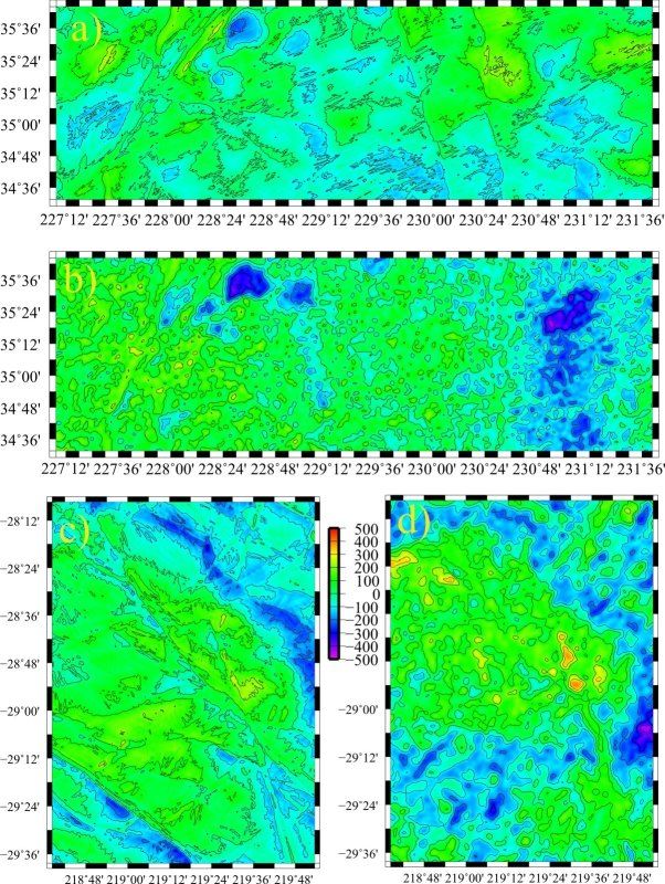
Photoclinométrie vs stéréoscopie
to quantify short-wavelength topographic roughness to design
radar instrument characteristics [4] or understand hazards to data set ∆x RMS dev.(100) dev.(1)
spacecraft landers. m m m m
e86-32 Z 32 106.2 7.7 0.21
ediss Z 55 87.2 8.5 0.27
eplains Z 21 51.4 7.1 0.22
erhad Z 65 75.3 5.6 0.20
etyre-33 Z 33 55.9 15.9 1.5
stéréo manan-80 Z 80 73.9 14.9 1.2
Satellite galliléens (Io,
Table 1: ‘Z’ denotes a stereo data set. ∆x is the pixel size;
Europe, Ganymède,
RMS and dev. are the RMS height and the RMS deviation as
defined by [9]. The RMS deviation at the specified wavelength
Callisto, ...) :
(100 m and 1 m, respectively) is derived by extrapolation from
the fitted roughness plots shown in Fig. 5.
PC
Pas d’autre moyen
que stéréoscopique
actuellement !
Résolution spatiale meilleure
pour la photoclinométrie !
stéréo PC
Nimmo, F. & Schenk, P. M., Stereo and Photoclinometric Comparisons and Topographic
Roughness of Europa, Lunar and Planetary Institute Science Conference Abstracts,
2008, 39, 1464-+
Figure 1: Topography for Erhad (a-PC b-stereo) and Ediss (c-
PC d-stereo) regions of Europa. Colour scale (in m) applies to Figure 2: a) Coherence between PC and S topography as aPlan • Définitions • Mesure de la topographie • Principe, incertitudes • Quelles interprétations planétologiques ?
Interprétations

• Comment comparer les altitudes ?
 • Hypsométrie
 • Pentes
 • loi d’échelle
Interprétations

• Comment comparer les altitudes ?
 • Hypsométrie
 • Pentes
 • Loi d’échelle
Comparaison Venus,
               Mars, Terre

• Etude rapide de deux publications
Sharpton, V. L. & Head, James W., I., Analysis of Regional Slope
                                                                   Aharonson, O.; Zuber, M. T. & Rothman, D. H., Statistics of Mars'
                                                                   topography from the Mars Orbiter Laser Altimeter: Slopes, correlations,
Characteristics on Venus and Earth, J. Geophys. Res., American
                                                                   and physical models, Journal of Geophysical Research, 2001, 106,
Geophysical Union, 1985, 90, 3733-3740
                                                                   23723-23736

• Questions:
      •
   Qu’est-ce qu’un hypsogramme ?
      •       Analyser les hyspogrammes des trois planètes
Vénus
Rayon équatorial
Terre
Rayon équatorial
Mars
Rayon équatorial
6 051,8 km 6 378,137 km 3 402,45 km
(0,95 Terre) (0,533 Terre)
Rayon polaire Rayon polaire Rayon polaire
6 051,8 km 6 356,7523142 km 3 377,4 km
(0,95 Terre) (0,533 Terre)
Périmètre équatorial Périmètre équatorial Périmètre équatorial
38 025 km 40 075,017 km 21 344 km
Superficie Superficie Superficie
4,60×10⁸ km² 510 067 420 km² 1,448×108 km²
(0,902 Terre) (0,284 Terre)
Volume Volume Volume
9,28×10¹¹ km³ 1,08321×10¹² km³ 1,638×1011 km³
(0,857 Terre) (0,151 Terre)
Comparaison
Masse Masse Masse
4,8685×1024 kg 5,9736×1024 kg 6,4185×10²³ kg
(0,815 Terre) (0,107 Terre)
Masse volumique moyenne Masse volumique moyenne Masse volumique moyenne
5,204×103 kg/m³ 5,515×103 kg/m³ 3,934×103 kg/m³
Gravité à la surface Gravité à la surface Gravité à la surface
physique
8,87 m/s² 9,780 m/s² 3,69 m/s²
(0,904 g) (0,99732 g) (0,376 g)
Vitesse de libération Vitesse de libération Vitesse de libération
10,361 km/s 11,186 km/s 5,027 km/s
Période de rotation Période de rotation Période de rotation
(jour sidéral) (jour sidéral) (jour sidéral)
(rétrograde) 0,99726949 d 1,025957 d
243,0185 d (23 h 56 min 4,084 s) (24,622962 h)
Vitesse de rotation Vitesse de rotation Vitesse de rotation
(à lʼéquateur) (à lʼéquateur) (à lʼéquateur)
6,52 km/h 1 674,364 km/h 868,220 km/h
Inclinaison de lʼaxe Inclinaison de lʼaxe Inclinaison de lʼaxe
-2,64° 23,4392° 25,19°
Albédo moyen Albédo moyen Albédo moyen
0,65 0,367 0,15
Température de surface Température de surface Température de surface
% •% Min. : 719 K (446°C) % •% Min. : 184,15 K = -89°C % •% Min. : 133 K = -140 °C
% •% Moy. : 737 K (464°C) % •% Moy. : 288 K = 15 °C % •% Moy. : 210 K = -63 °C
% •% Max. : 763 K (490°C) % •% Max. : 333 K = 60 °C % •% Max. : 293 K = 20°C
Pression atmosphérique Pression atmosphérique Pression atmosphérique
9,3219×10⁶ Pa 101 325 Pa 0,7-0,9×10³ Pa
(100 Terre) (0.001 Terre)the MOLA topographic profile data (18). topographic rise (10). However, Fig. 2 (see long-standing debate over the dominant con-
Downloaded from www.sciencemag.org on November 23, 20
Most of the northern lowlands is composed of also Fig. 6) shows that topographically Thar- tributors to the high elevations of the Tharsis
the Late Hesperian–aged (19) Vastitas Borea- sis actually consists of two broad rises. The region. A prominent ridge (containing Clari-
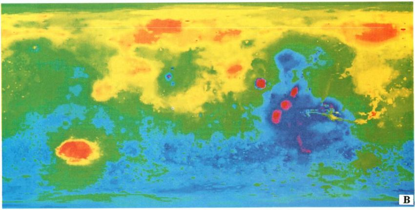
Comparaison Mars/Venus/Terre
SHARPTON AND HEAD: lis Formation,
IMPLICATIONS OF REGIONAL SLOPE DISTRIBUTION--VENUS AND EARTHwhich is flat and 7549
smooth (Fig. larger southern rise is superposed on the tas Fossae; Fig. 2) extends southward from
2), even at a scale as short as 300 m (Fig. 3). highlands as a quasi-circular feature that ex- the region of the Tharsis Montes, and then
The Amazonian-aged (19) Arcadia Forma- tends from "220°E to "300°E and from curves northeastward in a “scorpion tail” pat-
tion, which overlies the Vastitas Borealis "50°S to "20°N and spans about 107 km2 in tern. This arcuate ridge bounds Solis Planum,
Formation, is also smooth at large and small area. The highest portion of the southern rise a plateau within the southern rise. The ridge
scales, consistent with either a sedimentary contains the Tharsis Montes (Ascraeus, Pavo- contains an abundance of heavily cratered
(4, 20) or volcanic (21) origin for these nis, and Arsia). Eastward of the highest ter- Noachian material that has presumably es-
plains. In the southern hemisphere Noachian- rain but still elevated are the ridged plains of caped resurfacing by younger Tharsis volca-
aged (19) ridged plains form locally flat in- Lunae Planum (Fig. 2). The smaller northern nic flows because of its high elevation. It has
I I
tercrater deposits, whereas younger Hespe- rise is superposed on the lowlands and covers been suggested (25) that the termination of
Fig. 2. Maps of the global topography
of Mars. The projections are Mercator
to 70° latitude and stereographic at the
poles with the south pole at left and
north pole at right. Note the elevation
difference between the northern and
southern hemispheres. The Tharsis vol-
cano-tectonic province is centered near
the equator in the longitude range
220°E to 300°E and contains the vast
east-west trending Valles Marineris
canyon system and several major vol-
canic shields including Olympus Mons
(18°N, 225°E), Alba Patera (42°N,
252°E), Ascraeus Mons (12°N, 248°E),
Pavonis Mons (0°, 247°E), and Arsia
Mons (9°S, 239°E). Regions and struc-
o 180 tures discussed in the text include Solis
?70
Planum (25°S, 270°E), Lunae Planum
I
(10°N, 290°E), and Claritas Fossae
It (30°S, 255°E). Major impact basins in-
clude Hellas (45°S, 70°E), Argyre (50°S,
320°E), Isidis (12°N, 88°E), and Utopia
(45°N, 110°E). This analysis uses an
areocentric coordinate convention with
i,
east longitude positive. Note that color
scale saturates at elevations above 8
km.
ß
t% ß
ß ß ß
•.•.' . ,,
dilli' M
J ' I I
t;;3 .5 Z., B " E S
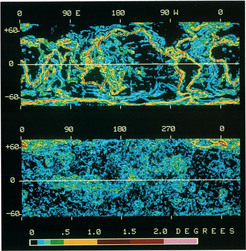
Plate 1. (Top) Regionalslopemap of earth depictingthe maximumslopemeasured1496 over 3ø by 3ø regions.The rangeof 28 MAY 1999 VOL 284 SCIENCE www.sciencemag.org
regional slope valuesfor earth, measuredat this scale,extendsfrom 0.0ø to 2.4ø. Standard error associatedwith slope
calculationsis 0.035ø [Sharptonand Head, 1985]. Each grid cell representsone degreeof latitude and one degree of
longitude (approximately 111.3 km at the equator). For regional slope less than 0.5ø, each map color representsa 0.1ø
slope increment; larger slope values are color-codedin 0.5ø increments(see color bar). (Bottom) Regional slope map of
Venus.The format, resolution,projection,and color scaleare equivalentto that of the top part. The range of regional Smith, D. E.; Zuber, M. T.; Solomon, S. C.; Phillips, R. J.; Head, J. W.; Garvin,
slopeson Venusextendsfrom 0.0ø to 2.4ø. At the equator,one degreeof latitude or longitudeequalsapproximately105.6
km.
J. B.; Banerdt, W. B.; Muhleman, D. O.; Pettengill, G. H.; Neumann, G. A.;
Lemoine, F. G.; Abshire, J. B.; Aharonson, O.; Brown, D. C.; Hauck, S. A.;
Sharpton, V. L. & Head, James W., I., Ivanov, A. B.; McGovern, P. J.; Zwally, H. J. & Duxbury, T. C.
Analysis of Regional Slope Characteristics on The Global Topography of Mars and Implications for Surface Evolution
Venus and Earth, J. Geophys. Res., American Science, 1999, 284, 1495-+
Geophysical Union, 1985, 90, 3733-3740Comparaison topographie
• Hypsométrie =
“mesure de la
topographie”
• Distribution
d’altitude
Aharonson, O.; Zuber, M. T. & Rothman, D. H., Statistics of Mars'
topography from the Mars Orbiter Laser Altimeter: Slopes, correlations,
and physical models, Journal of Geophysical Research, 2001, 106,
23723-237360.8 ,, [ .... [ .... [ .... [ ....
arth
0.6
0.4
0.2
0.0
i ß i I i i
-5 -2.5 0 3.5 5
p
0.8 :-' ' ' I .... I .... I .... I .... I .... s
Hypsométrie
q
Unloaded
0.6 s
-- arth - n
_ _
0.2 _
w
0.0 , I I [ I. ] I •/Y•/•/'41
] I i• i , i ] , i i! V
-5 -2.5 0 2.5 5 a
0.8
V
t
Venus V
0
• 0.4 t
p
c• 0.2
f
i
0 2.5 5 7.5 10 t
Elevation, km
Fig. 2. Differential hypsogramsfor the three topographic data e
setsusedin this analysis.All three data setsare of equivalentspatial
Sharpton, V. L. & Head, James W., I.,
and vertical resolution. Each plot illustrates the frequency of oc-
e
Analysis of Regional Slope Characteristics on
Venus and Earth, J. Geophys. Res., American currenceof surfaceelevationsgroupedin 100-m elevationincrements. V
Geophysical Union, 1985, 90, 3733-3740 For both terrestrial cases, 0.0-km elevation refers to sea level; for a
Venus,elevationsare referencedto a planetary radius of 6051.0 km. c
o
e
tDichotomie martienne ? • Nord • Sud • Faiblement cratérisée • Fortement cratérisée • Jeune • Agé • Faible altitude • Altitude élevée • Mécanisme interne : convection à degrée un • Océan magmatique : convection à degrée un • Un/plusieurs impacts géants
Interprétations

• Comment comparer les altitudes ?
 • Hypsométrie
 • Pentes
 • Loi d’échelle
Comparaison Venus,
               Mars, Terre
• Etude rapide de deux publications
                                                                   Aharonson, O.; Zuber, M. T. & Rothman, D. H., Statistics of Mars'
Sharpton, V. L. & Head, James W., I., Analysis of Regional Slope
                                                                   topography from the Mars Orbiter Laser Altimeter: Slopes, correlations,
Characteristics on Venus and Earth, J. Geophys. Res., American
                                                                   and physical models, Journal of Geophysical Research, 2001, 106,
Geophysical Union, 1985, 90, 3733-3740
                                                                   23723-23736

• Questions:
      •
   Analyser les pentes des trois planètes
      •      Quelles sont les implications sur les mécanismes
             externes/internes ?
ations increase systematicallywith elevation and equal or d
Venus vs Terre
exceedthe mean slopevaluesabove about 4.5 km. a
The specificboundariesof the major physiographicprov- d
inces of Venus [Masursky et al., 1980] do not appear to be in
tw
3736 SHARPTONAND HEAD: REGIONAL SLOPES--VENUSAND EARTH
s
el
Venus Mean Slope
Earth Mean Slope m
Ear[h Unloaded Mean Slope
0
o.a I .... I .... I .... I ' 't o.• ''' I .... I .... I .... I .... I"'
Tibetan
z
high • x continental Plateau re
highland plateaus
AVenus,elevationsare referencedto a planetary radius of 6051.0 km. curves' Venus has a significantlylarger percentage(66 + 1%)
of its total surface within this interval than does the unloaded
earth (47 + 1%). It is only for slopesgreater than about 0.3ø
Comparaison pente
that the differences between the Venus and earth distributions
The frequencydistribution of regional slopeson Venus and
earth are broadly similar, but they show wide variation in are lessenedslightly from 8 + 1% (loaded)to 6 + 1% (unload-
detail. ed). In order to interpretthe geologicalsignificance
of these
The modal regionalslopevalue for the earth curve is 0.0ø, data, information on the relationshipof slopesand elevations
is requiredso that slopescan be related to geologicand geo-
morphologicprovinces.
Regional Slope Frequency
Correlation of Mean Slope and Elevation
_
The relation between regional slope values and elevations
can be establishedby calculating the mean slope value for
30 '. Unloaded
Earth _ each 100-m elevation interval and displaying this together
_
Earth \ -
_ _
with the standard deviation associatedwith each mean slope
value. On Venus there is a distinct positive correlation be-
•
20 - \\•. ß
Venus -
_
tween mean slope and altitude (Figure 4). Lowest elevations
(-2.0 to -1.5 km) are characterizedby relativelyhigh mean
_
slopes,which are stronglyinfluencedby the presenceof linear,
steep-sidedtroughs(chasmata)in and around Aphrodite Terra
10 --
and Beta Regio [Schaber, 1982; Campbellet al., 1984]. This
zone is followed by an elevation range characterizedby con-
stant regional slope (about 0.1ø) extending to elevations of
approximately0.3 km. From 0.3 to 3.5 km the regionalslope
_
increasesconsistentlywith elevation. Above 3.5 km, mean re-
gional slopevarieswidely with elevation,but a distinctdepres-
0 0.1 0.2 0.3 0.4 0.5 0.6 0.7 0.8 0.9 1 sion in slopeis apparentbetween3.5 and 5.0 km correspond-
Slope, degrees ing to high plateau regions within westernAphrodite Terra,
Fig. 3. Regional slope frequency diagram for the three topo- Lakshmi Planum, and eastern Ishtar Terra. For elevations
graphic data sets used in this analysis.Each plot illustrates the fre- above 4.5 km the mean slopesare extremelyhigh and highly
quency of occurrenceof regional slopeswith data grouped such that
the first interval, plotted at 0.0ø, includesregional slopesin the range variable, reflecting the mountainous terrain characteristicof
of 0.0ø-0.07ø' all other intervalsare 0.035ø wide and are plotted at the theseelevations.Standard deviations of the mean slope values
minimum slopevalue.Seetext and appendixfor details. are only slightly lower than the slope value itself, suggesting
Aharonson, O.; Zuber, M. T. & Rothman, D. H., Statistics of Mars'
Sharpton, V. L. & Head, James W., I., Analysis of Regional Slope
topography from the Mars Orbiter Laser Altimeter: Slopes, correlations,
Characteristics on Venus and Earth, J. Geophys. Res., American
and physical models, Journal of Geophysical Research, 2001, 106,
Geophysical Union, 1985, 90, 3733-3740
23723-23736Venus,elevationsare referencedto a planetary radius of 6051.0 km. curves' Venus has a significantlylarger percentage(66 + 1%)
of its total surface within this interval than does the unloaded
earth (47 + 1%). It is only for slopesgreater than about 0.3ø
Comparaison pente
that the differences between the Venus and earth distributions
The frequencydistribution of regional slopeson Venus and
earth are broadly similar, but they show wide variation in are lessenedslightly from 8 + 1% (loaded)to 6 + 1% (unload-
detail. ed). In order to interpretthe geologicalsignificance
of these
The modal regionalslopevalue for the earth curve is 0.0ø, data, information on the relationshipof slopesand elevations
is requiredso that slopescan be related to geologicand geo-
morphologicprovinces.
Regional Slope Frequency
Correlation of Mean Slope and Elevation
_
The relation between regional slope values and elevations
can be establishedby calculating the mean slope value for
30 '. Unloaded
Earth _ each 100-m elevation interval and displaying this together
_
Earth \ -
_ _
with the standard deviation associatedwith each mean slope
value. On Venus there is a distinct positive correlation be-
•
20 - \\•. ß
Venus -
_
tween mean slope and altitude (Figure 4). Lowest elevations
(-2.0 to -1.5 km) are characterizedby relativelyhigh mean
_
slopes,which are stronglyinfluencedby the presenceof linear,
steep-sidedtroughs(chasmata)in and around Aphrodite Terra
10 --
and Beta Regio [Schaber, 1982; Campbellet al., 1984]. This
zone is followed by an elevation range characterizedby con-
stant regional slope (about 0.1ø) extending to elevations of
approximately0.3 km. From 0.3 to 3.5 km the regionalslope
_
increasesconsistentlywith elevation. Above 3.5 km, mean re-
gional slopevarieswidely with elevation,but a distinctdepres-
0 0.1 0.2 0.3 0.4 0.5 0.6 0.7 0.8 0.9 1 sion in slopeis apparentbetween3.5 and 5.0 km correspond-
Slope, degrees ing to high plateau regions within westernAphrodite Terra,
Fig. 3. Regional slope frequency diagram for the three topo- Lakshmi Planum, and eastern Ishtar Terra. For elevations
graphic data sets used in this analysis.Each plot illustrates the fre- above 4.5 km the mean slopesare extremelyhigh and highly
quency of occurrenceof regional slopeswith data grouped such that
the first interval, plotted at 0.0ø, includesregional slopesin the range variable, reflecting the mountainous terrain characteristicof
of 0.0ø-0.07ø' all other intervalsare 0.035ø wide and are plotted at the theseelevations.Standard deviations of the mean slope values
minimum slopevalue.Seetext and appendixfor details. are only slightly lower than the slope value itself, suggesting
Aharonson, O.; Zuber, M. T. & Rothman, D. H., Statistics of Mars'
Sharpton, V. L. & Head, James W., I., Analysis of Regional Slope
topography from the Mars Orbiter Laser Altimeter: Slopes, correlations,
Characteristics on Venus and Earth, J. Geophys. Res., American
and physical models, Journal of Geophysical Research, 2001, 106,
Geophysical Union, 1985, 90, 3733-3740
23723-23736Interprétations • Comment comparer les altitudes ? • Hypsométrie • Pentes • Loi d’échelle
Symétrie/invariance
          d’échelle
• von Koch
• Mandelbrot
Symétrie ou
invariance
d’échelle
règle
• Mesure de la taille totale
dépend de la taille de la règle
taille
totale
taille de la règleSymétrie ou
invariance
d’échelle
règle
• Mesure de la taille totale
dépend de la taille de la règle
taille
totale
taille de la règleSymétrie ou
invariance
d’échelle
règle
• Mesure de la taille totale
dépend de la taille de la règle
taille
totale
taille de la règleTopographie E598
distance (km) TURCOTTE: TOPOGRAPHY AND GE
104 103
iOII
i•x ! i i i I The
5
where
• Terre, Mars, Lune :
fractal
{0Iø 1967] w
x a mea
Processus brownien cycles
the nu
coastlin
(D=1.5) Am
o Earth
Oo +
n o +
• Venus : croute Variance
For a t
a Venus ++ The
x Mars tempo
includ
moins rigide car + Moon random
will co
haute température IO8
geoid.
examp
10-4 k cycles
km
I0-a (or ge
spheri
Fig. 1. Energy spectraldensityof topographySt as a function of for one
wave number k. Ther
fractal
Turcotte, D. L., A fractal interpretation of topography and geoid the frac
spectra on the Earth,Moon, Venus, and Mars, jgr, 1987, 92, 597-+
over which data are includedin the expansion.With Xo= 2rrRo are con
we find over a
! has th
mostti
St(k/)
--271'Rø3
Z (C]/mq-
Slim)
m=0
(7)Comparaison Venus,
Mars, Terre
• Etude rapide de publication
Aharonson, O.; Zuber, M. T. & Rothman, D. H., Statistics of Mars'
topography from the Mars Orbiter Laser Altimeter: Slopes, correlations,
and physical models, Journal of Geophysical Research, 2001, 106,
23723-23736
• Question :
•Quels arguments géométriques en faveur d’une
différence Nord/Sud sur Mars ?Océans ?
Indices topographiques :
• Nord et Sud cratérisé à petite
échelle
• Seulement Nord compatible avec
une processus de dépôt
Aharonson, O.; Zuber, M. T. & Rothman, D. H., Statistics of Mars'
topography from the Mars Orbiter Laser Altimeter: Slopes, correlations,
and physical models, Journal of Geophysical Research, 2001, 106,
23723-23736Plaines Nord de Mars
• Cratères enfoui au Nord
• Indice MOLA + echo
radar de subsurface
• Age plus vieux
recouvert de coulée de
lave + océansOcéans ?
Head, J. W.; Kreslavsky, M.; Hiesinger, H.; Ivanov, M.; Pratt, S.;
Seibert, N.; Smith, D. E. & Zuber, M. T., Oceans in the past history of
mars: Tests for their presence using Mars Orbiter Laser Altimeter
(MOLA) data, Geophysical Research Letters, 1998, 25, 4401-4404Interprétations • Processus de surface (érosion, sédimentation, ...) • Processus internes (tectonique des plaques, ...)
Référence
Planetary sciences / Imke de Pater, and Jack J. Lissauer,... . -
Cambridge, U. K. : Cambridge university press ,

 •   ISBN 0-521-48219-4. - ISBN 978-0-521-48219-6.

 •   Orsay-BU Sciences, Rez-de-chaussée

 •   Cote : 523.4 PAT pla

 •   No : 9530338349
Vous pouvez aussi lire