Control of three-dimensional wakes using evolution strategies
←
→
Transcription du contenu de la page
Si votre navigateur ne rend pas la page correctement, lisez s'il vous plaît le contenu de la page ci-dessous
C. R. Mecanique 333 (2005) 65–77
http://france.elsevier.com/direct/CRAS2B/
High-Order Methods for the Numerical Simulation of Vortical and Turbulent Flows
Control of three-dimensional wakes using evolution strategies
Philippe Poncet a,∗ , Georges-Henri Cottet b , Petros Koumoutsakos c
a Laboratoire MIP, département GMM, INSA, complexe scientifique de Rangueil, 31077 Toulouse cedex 4, France
b Laboratoire LMC-IMAG, BP 53, 38041 Grenoble cedex 9, France
c Institute of Computational Science, Swiss Federal Institute of Technology, 8092 Zürich, Switzerland
Available online 4 January 2005
Abstract
We investigate three-dimensional cylinder wakes of incompressible fully developed flows at Re = 300, resulting from control
induced by tangential motions of the cylinder surface. The motion of the cylinder surface, in two dimensions, is optimized using
evolution strategies, resulting in significant drag reduction and drastic modification of the wake as compared to the uncontrolled
flow. The quasi-optimal velocity profile obtained in 2D is modified by spanwise harmonics and applied to 3D flows. The results
indicate important differences in the flow physics induced by two and three dimensional control strategies. To cite this article:
P. Poncet et al., C. R. Mecanique 333 (2005).
2004 Académie des sciences. Published by Elsevier SAS. All rights reserved.
Résumé
Stratégies évolutionnaires pour le contrôle des sillages tridimensionnels. On s’intéresse aux sillages de cylindres in-
compressibles dont la tridimensionnalité est totalement développée à Re = 300, obtenus suite à un contrôle exercé par des
mouvements tangentiels à la surface du corps. Les mouvements de surface sont optimisées par des stratégies évolutionnaires, et
ont pour conséquence une réduction subtantielle du coefficient de traînée et une modification importante du sillage par rapport
à l’écoulement non contrôlé. Le profil de vitesse quasi-optimal obtenu en 2D est modifié par des harmoniques dans la direction
axiale, et appliqué à un écoulement 3D. Les résultats indiquent d’importantes différences dans la physique de l’écoulement
selon la nature 2D ou 3D du contrôle. Pour citer cet article : P. Poncet et al., C. R. Mecanique 333 (2005).
2004 Académie des sciences. Published by Elsevier SAS. All rights reserved.
Keywords: Computational fluid mechanics; Evolution strategy; Three-dimensional wake
Mots-clés : Mécanique des fluides numérique ; Stratégie évolutionnaire ; Sillage tridimensionnel
* Corresponding author.
E-mail addresses: philippe.poncet@insa-toulouse.fr (P. Poncet), georges-henri.cottet@imag.fr (G.-H. Cottet), petros@inf.ethz.ch
(P. Koumoutsakos).
1631-0721/$ – see front matter 2004 Académie des sciences. Published by Elsevier SAS. All rights reserved.
doi:10.1016/j.crme.2004.10.007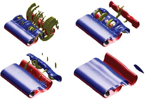
66                                    P. Poncet et al. / C. R. Mecanique 333 (2005) 65–77

Version française abrégée

    Cette Note présente une approche numérique de quelques méthodes de contrôle du coefficient de traînée d’un
sillage créé derrière un cylindre circulaire, en agissant sur la vitesse tangentielle à la surface du cylindre.
    On considère les équations de Navier–Stokes 2D et 3D pour un fluide incompressible s’écoulant autour d’un
cylindre circulaire de longueur infinie de diamètre D :
       ∂u                             ∇p
            + (u · ∇)u − νu = −
        ∂t                              ρ
en formulation vitesse–pression, et
       ∂ω
             + (u · ∇)ω − (ω · ∇)u − νω = 0
        ∂t
en formulation vitesse-tourbillon, sur un domaine Ω cylindrique externe. La vitesse vérifie ∇ · u = 0 (incompressi-
bilité), et sa condition à l’infini est U∞ ex . On recherche des solution L-périodiques (où L = 2πD en pratique) afin
de prendre en compte la longueur infinie du cylindre. Le contrôle s’opère par l’intermédiaire de la fonction Vslip
dans la condition aux limites en vitesse u(x, t) = Vslip (x, t) eθ , qui représente un champ de vitesses tangentielles.
La fonction Vslip sera appelée profil de vitesse. L’énergie cinétique moyenne adimensionnée mise en jeu par un tel
contrôle est alors
                               T
          ∗          1
       Ec =         2 σ (∂Ω)
                                     Vslip (t)2 ds dt
               2T U∞
                               0 ∂Ω
où σ (∂Ω) la mesure du cylindre (πD en 2D et πLD en 3D).
   Le critère à optimiser est le coefficient de traînée (voir [3]) défini par

                  ν           ∂ωz
      CD = − 2              r      + ωz sin θ ds
               U∞ RL           ∂r
                          ∂Ω
   Des calculs préliminaires montrent (voir [2]) que pour un profil particulier (invariant dans la direction axiale du
cylindre), le carré de la diminution du coefficient de traînée est propotionnel à l’énergie mise en jeu par le contrôle.
Par conséquent, un critère perspicace pour mesurer l’efficacité d’un profil est par exemple
               0 −C
              CD      D
      Eff =
                  Ec∗
où CD 0 est le coefficient de traînée du sillage sans contrôle (valant 1.382 en 2D pour un nombre de Reynolds de 300).

    Dans un premier temps, on considère les cylindres en rotation oscillante dans le cas 2D, pour plusieurs nombres
de Reynolds entre 200 et 1000 (cf. [3,11,10]). L’algorithme numérique est une méthode de type Vortex-in-Cell
hybride intégrant les équations de Navier–Stokes en formulation vitesse-vorticité (voir [4,3]). Il apparaît que de
telles stratégies sont très coûteuses en énergie et difficiles à mettre en pratique, l’efficacité maximale étant de 0.3
(atteinte pour Re = 1000).
    Dans un second temps, toujours pour des simulations bidimensionnelles, on cherche un profil de vitesse optimal
sur le bord du cylindre. On considére à présent uniquement des profils stationnaires. Cela revient à minimiser la
fonctionnelle


                 T
                1
       J (c) =          CD 2 (c, t) + Yc, c dt
                  T
                    0
où T est l’horizon en temps de contrôle (le systéme est quasiment périodique), et c le vecteur des paramètres de
contrôle, ici dans R16 , représentant les vitesses tangentielles sur 16 arcs de cercles de même longueur décrivant le
P. Poncet et al. / C. R. Mecanique 333 (2005) 65–77 67
cylindre (la matrice de régularisation/pénalisation Y est nulle dans toute la présente note). La formulation vitesse-
pression est utilisé dans ce cas, en utilisant le schéma numérique de [1,12] pour Re = 500. La minimisation est
obtenue par l’algorithme génétique défini dans [1]. On obtient ainsi un profil efficace et très peu coûteux en énergie.
Le profil est néanmoins peu régulier ce qui rend délicates les simulations tri-dimensionnelles (à cause de la faible
longueur caractéristique des instabilités hydrodynamiques 3D).
On est donc amené dans un troisième temps à régulariser le profil obtenu ci-dessus en interpolant la fonction de
contrôle (vitesses constantes par morceaux) par une fonction régulière et symétrique. On obtient ainsi une méthode
légèrement moins coûteuse en énergie et plus robuste.
Enfin, ce profil est rendu tridimensionnel en superposant des fonctions sinusoïdales calées sur trois harmoniques
des instabilités tri-dimensionnelles dans la direction axiale. Le profil totalement 3D est ainsi défini par un jeu de 4
paramètres C. On peut alors étudier l’impact de la tridimensionnalité du contrôle sur la réduction de coefficient de
traînée et sur le critère d’efficacité.
Deux phénomènes sont mis en évidence. D’une part, l’ajout de tridimensionnalité dans le contrôle permet d’ob-
tenir un coefficient de traînée plus faible pour la même quantité d’énergie impliquée dans le contrôle. Il semble par
ailleurs que la tridimensionnalité est d’autant plus efficace que la longueur d’onde est petite (pour les paramètres de
la présente note). D’autre part, il existe une énergie critique au dessous de laquelle la tridimensionnalité n’apporte
pas de gain. L’identification d’une telle énergie est un défi pour ce qui concerne les futurs développements de ces
méthodes d’optimisation. Elle caractérise une transition dans la physique du problème qui devra être élucidée.
1. Introduction
The efficient control of wakes is of paramount importance in the aircraft and automobile industry. Depending
on the particular application, wake control can have various goals and can be achieved either by passive or active
strategies. Passive control is mostly achieved by shape optimisation and often results in the addition of appendices
like foilers or riblets to the surface of the obstacle. Active control involves imparting energy to the flow by means
of actuators (e.g. mass transpiration) on the surface of the obstacle.
While passive control strategies have led to important improvements in the design of automobiles and aircraft
in the last decades, nowadays this approach shows its limits, mostly due to design considerations. Active control
strategies are becoming ever more important as they can circumvent some of these difficulties and in addition they
provide additional flexibility to tackle new stringent regulations on pollutant emissions. These control strategies,
beside the technology issues that they raise, are very demanding in terms of simulation and optimisation tools as
they often involve unsteady simulations. Three-dimensional wakes are still a very challenging field for simulation
methods, because of the complex unsteady features of the flows.
To illustrate active control of wakes in this article we implement a high order vortex-in-cell scheme and we
apply it to the control of three-dimensional wakes behind a 3D circular cylinder using open-loop strategies. We
first describe a two-dimensional optimisation using surface ‘belt-like’ actuators obtained with the clustering genetic
algorithm developed in [1]. The optimised two-dimensional velocity profile of the actuators is then smoothed and
used as a 2D control profile on the three dimensional surface to control three-dimensional wakes. The full 3D
control is finally introduced using stationary three-dimensional tangential velocity distributions and resulting in
significant drag reduction.
2. Governing equations and diagnostics
The wake of a viscous flow around a cylinder can be computed by solving numerically the full three-dimensional
Navier–Stokes equations in an external cylindrical domain Ω of radius R in its velocity-vorticity formulation for68 P. Poncet et al. / C. R. Mecanique 333 (2005) 65–77
Sections 3, 5 and 6:
∂ω
+ (u · ∇)ω − (ω · ∇)u − νω = 0 (1)
∂t
and in its velocity–pressure for Section 4:
∂u ∇p
+ (u · ∇)u − νu = − (2)
∂t ρ
where the velocity field u satisfies
∇·u=0 (3)
for both the formulations. Here, for all three-dimensional computations, solutions are spanwise L-periodic. The
no-slip boundary condition on the cylinder wall requires that the fluid and solid velocities are equal on the body
surface:
u(x, t) = Vslip (x, t)eθ (4)
for x ∈ ∂Ω (i.e. r = R), where Vslip may be non-constant in time and space.
Two important non-dimensional parameters of the flow are the Reynolds and Strouhal numbers, defined respec-
tively by
U∞ D fD
Re = and St =
ν U∞
where U∞ is the far field velocity, D the cylinder diameter (R = D/2 will denote the radius), ν the kinematic
viscosity and f the natural flow frequency. The non-dimensional time is defined as:
t ∗ = U∞ t/R
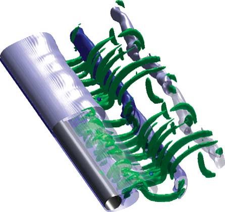
The flow becomes fully three-dimensional when Re 190 as manifested by vorticity isosurfaces (along with
drag/lift curves) in Fig. 1. The drag coefficient CD and the lift coefficient CL of the flow are given as sums of
friction and pressure coefficients:
CD = CDF + CDP and CL = CLF + CLP (5)
Fig. 1. Effect of three-dimensionality on drag and lift coefficients at Re = 300 (left picture) and vorticity isovalues of post-transient
three-dimensional flow (right picture, from [4]).P. Poncet et al. / C. R. Mecanique 333 (2005) 65–77 69
where the friction coefficients are defined by:
ν ν
CDF = − 2 ωz sin θ ds, CLF = 2 ωz cos θ ds
U∞ RL U∞ RL
∂Ω ∂Ω
and the pressure coefficients by:
ν ∂ωz ν ∂ωz
CDP = − 2 r sin θ ds, CLP = 2
r cos θ ds
U∞ RL ∂r U∞ RL ∂r
∂Ω ∂Ω
The present work on wake optimisation aims at minimizing the drag coefficient without affecting the average lift
of the flow. Note that in two dimensions, one has to remove L and integrate with respect to R dθ .
The mean energy involved in the control, i.e. required to provide the tangential boundary conditions, can be
related to a kinetic energy quantity:
T
1
Ec = Vslip (t)2 ds dt (6)
2T
0 ∂Ω
but this quantity is physically massic (i.e. per unit of mass) and is defined over a surface. A more pertinent quantity,
which will be called non-dimensional energy from now on, is its non-dimensional formulation
T
1
Ec∗ = 2
Vslip (t)2 ds dt (7)
2T U∞ σ (∂Ω)
0 ∂Ω
where σ (∂Ω) is a measure of the body: σ (∂Ω) = LπD is the body surface in 3D, while σ (∂Ω) = πD in 2D.
Preliminary computations using a 2D profile, for a Reynolds number Re = 300, show that for sufficiently large
values of Vslip (see Section 4) the mean-drag reduction is basically proportional to Vslip . Since energy is pro-
portional to Vslip 2 , mean-drag reduction behaves as a square root regression of energy: this property is shown in
[2] for a 2D profile, and work is underway to investigate further this observation for 3D profiles. This seems thus
interesting to define the strategy efficiency by the ratio between drag reduction and the square root of energy, that
is to say:
Eff = (CD0
− CD )/ Ec∗ (8)
where CD 0 the uncontrolled drag coefficient (1.382 at Re = 300). This quantity consequently represents the most
objective way to study the dependency of drag reduction with respect to the shape of tangential velocity field.
3. Body rotation
For the rotating body simulations, as well as for Sections 5 and 6, we consider a hybrid Vortex-In-Cell method,
in the spirit of [3]. This numerical scheme is based on a Lagrangian particle approximation of the vorticity field
ω(t). A particle carries elements of vorticity, volumes and locations (ωp , vp , xp ), and these quantities satisfy the
following system of differential equations:
dxp dωp
= u(xp ), = (ω · ∇u)(xp ) + νω(xp ) (9)
dt dt
while volumes remain constant due to the incompressibility. The no-slip condition u(t) = Vslip (t)eθ , is satisfied by
means of a flux of vorticity [4].
Derivatives are calculated using a 4th-order scheme (usually centered, and biased close to walls), time integra-
tion is performed with a fourth-order Runge–Kutta step, interpolation and periodic remeshing are third-order, diffu-70 P. Poncet et al. / C. R. Mecanique 333 (2005) 65–77
sion is 2nd order. This convection/diffusion step is followed by a flux of vorticity from the cylinder surface, thus en-
forcing the no-slip condition (using the integral technique presented in [4,14]). The whole fractional step algorithm
solving Eq. (1) is globally second order. This numerical method is taking implicitly into account transport terms
and it has no stability condition for the convective time step. Thus, with the present numerical method, one can use
long time steps providing an efficient tool to compute the large time scales behaviour of three-dimensional flows.
This technique has been successfully used on various two-dimensional domains and simple three-dimensional
geometries [5,6], and more recently on cylindrical geometry [7,4,3,8]. This scheme is extended to arbitrary domains
using immersed boundary techniques with interesting preliminary results [4].
The oscillatory rotation of the body as a drag reduction mechanism was first shown in experiments by Toku-
maru and Dimotakis in the early 90s, at Re = 1.5 × 10⁴ (cf. [9]). It has been recently followed by accurate
two-dimensional numerical simulation [10,11] for Reynolds numbers up to 1000. The three-dimensional aspects
of the wake behind a cylinder in oscillatory rotation have been since studied in [3].
The cylinder rotations considered herein, consist of following a point on the cylinder at angle θ (t) satisfying
θ (t) = −A cos(2πfc t) (10)
where fc is the control frequency and A the rotation amplitude. A usual non-dimensional frequency is the forced
Strouhal number SF (often chosen among St multiples) defined as SF = fc D/U∞ . One obtains
θ (t) = −A cos(πSF U∞ t/R) = −A cos(πSF t ∗ )
and consequently the tangential velocity on the body (i.e. for r = R) is given by
dθ
Vslip (t ∗ ) = R = AπSF U∞ sin(πSF t ∗ ) (11)
dt
and its mean non-dimensional value is Vslip (t ∗ )/U∞ = AπSF /2. The non-dimensional mean kinetic energy in-
volved in such a control is then
T
∗ 1
Ec = 2 σ (∂Ω)
Vslip (t)2 dl dt = (AπSF )2 /2 = A2 π 2 SF2 /2 (12)
2T U∞
0 ∂Ω
where T is the rotation period and σ (∂Ω) = 2πR the circle measure. The present computations are run with an
amplitude A = π/2, which means Ec∗ = π 4 SF2 /8.
Fig. 2 shows the drag reduction with respect to Ec∗ for three Reynolds numbers: Re = 200 from [11], Re =
500 from [3] and Re = 1000 from [11]. From these results we can observe that using cylinder rotation as drag
Fig. 2. Drag reduction −CD due to cylinder rotation versus non-dimensional energy Ec∗ at various Reynolds numbers (left picture,
Re = 200, 500 and 1000 from bottom to top, 2D simulations, A = π/2), and typical stream contours obtained for this flow (right picture,
from [3]).P. Poncet et al. / C. R. Mecanique 333 (2005) 65–77 71
coefficient control is expensive in energy, and furthermore is difficult to bring to realistic engineering, especially
for aeronautics concerns. The efficiency coefficient Eff is at most 0.3 for all the simulations plotted on Fig. 2.
4. A Clustering Genetic Algorithm for flow optimization
The Clustering Genetic Algorithm (CGA) was introduced in [1] for the control of the two-dimensional flow past
a circular cylinder at Re = 500. The cylinder surface is subdivided in 16 equally sized segments (see Fig. 3) and
each segment is allowed to move tangentially to the cylinder surface, with all the segments moving with different
but steady velocities.
The present CGA has not been implemented on a vortex method. The Navier–Stokes equations are discretized
on an O-grid using a staggered, second-order central-difference method in generalized coordinates (stretched as
cosh in radius, see [12]). The radius/angle resolution used was up 160 × 320 for 30 cylinder radius and the time
step was 3 × 10⁻³ .
An optimal regulation problem (2) can be set up by considering the functional
T
1 2
J (c) = CD (c, t) + Yc, c dt (13)
T
0
where c is the input vector in [−1, 1]16, which represents the velocities on the 16 panels, T is the time horizon
considered, which in the present case was four times the Strouhal period U∞ /(f R) of the uncontrolled flow, and Y
Fig. 3. Belt configuration (top left picture), resultant drag coefficient for the best population member (top right picture, — : all the actuators,
- - : only the four most influential) and population histogram (bottom), from [1].72 P. Poncet et al. / C. R. Mecanique 333 (2005) 65–77
is the penalty input weighting matrix (Y ≡ 0 in all the present article). The functional J , subjected to the constraints
(2)–(4) must be minimized with respect to c in order to minimize the drag.
The parameters of the optimisation involve the amplitude of the velocities on the cylinder surface and they are
optimised using a CGA proposed in [1]. The CGA operates on a parameter population in which an input vector c
consists of one population member. Three operators are defined to modify the population members:
• Recombination/crossover, which generates new trial solution points (offsprings), using some elements drawn
from the population;
• Mutation, which randomly changes some of the offsprings’ components;
• Selection, which chooses the population elements that will be used by the crossover.
For each population element a fitness function is defined, measuring how close a given solution is to the de-
sired goal. Based on their fitness, the old population members are compared with the newly generated ones, and
the solutions with the better fitness constitute the new population members. In this way, iterating the selection–
crossover–mutation process, the population evolves toward the desired optimal solution. The CGA is a real coded
GA that is particularly suitable for finding clusters of good solutions [1], a desirable scheme when smooth, non-
single point minima are sought. A variable mutation operator, depending on the local fitness value and on the global
success history of the population, allows the population to avoid local minima. For more details, see [1].
The population histogram of velocities, obtained by this algorithm, is plotted on Fig. 3. The best population,
defined by highest frequencies, lead to a drag reduction of 0.741, and satisfies
16
ci2 δli = 1 (14)
i=1
∗
where ci and δli are velocity and length of panel i. The non-dimensional energy is then Ec = 0.08 and the effi-
∗
ciency defined in Eq. (8) is then −CD / Ec = 2.62. It can be observed that most parameters are not clustered,
an indication of the fact that they have little influence on the fitness function. The most evident clustering can be
observed for the velocities assigned to actuators 3–4 and 13–14, which contain the separation point of the uncon-
trolled cylinder.
It turns out these four actuators can be used alone and make one expect a significant drop of drag coefficient.
Indeed, in this case the drag coefficient decreases down to 0.775, which is 4.6% higher than previously when all
actuators are used, but the energy involved is only 0.234; thus population clustering leads to a much more efficient
control. This clustering technique leads to a substantial gain of efficiency, which reaches 3.46.
This result will be used as a starting point for control of three-dimensional flows in next section.
5. Two-dimensional control for 3D flows
In the following implementations of control strategy, it was important to avoid discontinuities of velocity that
would interact with natural three-dimensional instabilities of the flow. This led us to use a smooth function able to
fit in a reasonable way the values obtained on actuators 3–4 and 13–14 (see Fig. 4 for instance). One then obtains
the following function:
3.2θ 3
f (θ ) = − sin (15)
3 + θ 10
defined over [−π, π]. Its extrema are ±0.723 and its Euclidean norm is numerically:
π
f (θ )2 dθ 0.49435 (16)
−πP. Poncet et al. / C. R. Mecanique 333 (2005) 65–77 73
Fig. 4. Velocities related to the best population obtained by the GA using all belt actuators (left picture), and shape of function f , smooth
approximation of these velocities (right picture), with its extrema at ±0.723.
Fig. 5. Effect of 2D control (C = 1) on drag coefficient (on the left). Snapshots of the 3D flow (on the right), contour of isovorticity (positive,
negative and transverse vorticity). Dotted lines mean: ——— : 2D without control, – – – : 3D without control, - - - - - : 2D with control,
......... : 3D with control.
This profile is very comparable in terms of energy to the profile defined by the best clustered population mentioned
above, and is smooth, symmetric, and is by far cheaper in energy than the profile obtained with the non-clustered
populations.
If velocity on the body is Vslip (θ ) = CU∞ f (θ ), then the non-dimensional energy involved in this control is
L π π
1 C2
Ec∗ = 2
Vslip (θ ) R dθ dz =
2
f (θ )2 dθ (17)
4πRLU∞ 4π
0 −π −π
The coefficient C adjusts the velocity field, and the case C = 1 can be considered as a smooth approximation of
the velocity profile obtained by the clustering genetic algorithm, and is only 5.6% times as expensive as the best
clustered population. The drag coefficients obtained for such a profile are plotted on Fig. 5, for 2D and 3D flows.74 P. Poncet et al. / C. R. Mecanique 333 (2005) 65–77
As mentioned in Section 2, one can define the strategy efficiency in 3D by
0
Eff = CD − CD / Ec∗
where CD 0
is the two-dimensional uncontrolled drag coefficient (1.382 at Re = 300), because three-dimensionality
tends to disappear when high-energy control is performed (see [13] and Fig. 5). Indeed, preliminary computations at
Re = 300 show that the mean-drag reduction is basically proportional to C, and since energy is proportional to C 2 ,
mean-drag reduction behaves as a square root regression of energy (see [2]). It thus expected that Eff depends only
on the shape of velocity distribution and not on the global amplitude |C| or C2 in a more general way (at least
for large values of C).
This efficiency criteria shows us that for C = 1, one gets a drag reduction of 0.747 and an efficiency of 3.77.
The genetic algorithm using all belt actuators has an efficiency of 2.62 with a drag reduction of 0.741, while the
clustered population leads to an efficiency of 3.46, with a drag reduction of 0.668. On the one hand, the smooth
profile provides a comparable drag reduction, and uses less energy because function f has less significant values
than the best population of the Genetic Algorithm (the viscosity used is also larger). One the other hand, when
compared to the clustered population, the smooth profile leads to a slightly better drag reduction with a similar
energy, thus a slightly better but similar efficiency. Nevertheless, one may notice that these comparisons have been
made between 2D flows at Re = 500 (for the GA and CGA) and Re = 300 for 3D flows.
Furthermore, the three-dimensionality of the flow has no effect on the efficiency because one can observe (see
[13]) that the three-dimensionality is suppressed by this kind of control (see Fig. 5), and the same drag coefficient
is achieved, whether the initial flow is 2D or 3D.
6. Three-dimensional control using mode combination
To account for spanwise variations, in a general formulation, one can consider the following vector of size n + 1
C0
C1
C=
... (18)
Cn
The azimuthal tangential velocity profile on the body is then given by
1
2 sin(2πz/L1 )
Vslip (θ, z) = f (θ )U∞ C ·
2 sin(2πz/L2 )
(19)
..
.
2 sin(2πz/Ln )
where L1 , L2 , . . . , Ln are n wavelengths, usually sub-harmonics of the spanwise length L. The spanwise invariant
coefficient is associated to L0 = ∞ and is often called mode 0.
The non-dimensional energy involved in the control is then
Lπ π
1 1 1
Ec∗ = 2
Vslip (θ, z) R dθ dz =
2
C22 f (θ )2 dθ = C22 f 2 (20)
4πRLU∞ 4π 2
0 −π −π
whatever the wavelength values Li .P. Poncet et al. / C. R. Mecanique 333 (2005) 65–77 75
Fig. 6. Left picture: Drag reduction with respect to non-dimensional energy involved in the control. Right picture: Efficiency Eff given by
formula (8). Numbers mean: 1: Best population obtained by the Genetic Algorithm, applied to a 2D flow. 2: Best clustered population ob-
tained by the Genetic
√ Algorithm, applied to a 2D flow. 3: 2D profile, C = 1, applied to a 3D flow. 4: Combination
√ between 2D and mode A,
C = (2, 1, 0, 0)/ 5, applied to a 3D flow. 5: Combination between 2D and L2 = π D/2, C = (2, 0, 1, 0)/ 5, applied to a 3D flow.
The present computations use four control parameters, that is to say:
C0
C
C= 1 (21)
C2
C3
In the present case, cylinder spanwise length is L = 2πD, and control wavelengths are Li = L/2i . We will base
our control strategies on the natural three-dimensional instabilities, i.e. mode A and B instabilities, that naturally
appear in cylinder wakes (see [3,8] and the references therein). The closest possible wavelength to mode A is L1 ,
while L3 = πD/4 excites mode B, the dominant instability at Re = 300. Eq. (19) can then be written:
1
2 sin(2z/D)
Vslip (θ, z) = f (θ )U∞ C · (22)
2 sin(4z/D)
2 sin(8z/D)
and the energy used is given by Eq. (20).
A few computations in the case C2 = 1 have been performed in [13], and concluded two main results. On the
one hand, there is no drag reduction when mode 0 is not present, that is to say when C0 = 0. On the other hand,
drag reduction is larger when three-dimensionality is slightly present in the control (i.e. when C1 , C2 and/or C3 are
non zero and small enough) than when it is not (i.e. when they are all zero, see points 1/2/3 and 4/5 on left part of
Fig. 6 for instance).
This implies that there is an optimal combination of modes for the drag reduction. In the near future, full 3D
Optimisation Algorithms will be implemented to identify this optimal combination.
Moreover, the right part of Fig. 6 compares the efficiency for pure 2D control and mixed 2D–3D control, for
the same energy√involved (C2 = 1). It√is shown that combination between mode 0 and one 3D mode, here
C = (2, 1, 0, 0)/ 5 and C = (2, 0, 1, 0)/ 5, is always more efficient than the pure 2D control C = (1, 0, 0, 0).
Indeed, this last 3D case leads to an efficiency of 4.44.76 P. Poncet et al. / C. R. Mecanique 333 (2005) 65–77
Fig. 7. Final Drag coefficient with respect to α/ 1 + α 2 , for β = 0.25 (2) and β = 1 (). Right picture is a zoom of left picture, showing only
low-energy strategy (β = 0.25).
We remark also that the physics of the flows are different for small and large values of C. Since
√ among the
computations above, the combination between 2D and L2 = πD/2 defined by C = (2, 0, 1, 0)/ 5 is the most
efficient, one can consider the following weighted strategy:
(1, 0, α, 0)
C=β √ (23)
1 + α2
With such a notation, the control amplitude
√ is C2 = β. The strategy is two-dimensional (case ‘2’ on Fig. 6) when
α = 0, and the case C = (2, 0, 1, 0)/ 5 (case ‘4’ on Fig. 6) corresponds to α = 1/2 and β = 1.
One has already shown that for β = C2 = 1, there exists an optimal strategy C. Moreover, when β = C2 =
1/4, the final drag coefficient has been computed for
α = {0, 1/10, 3/10, 1/2, 1}
It appears that, in this range and for this energy, adding three-dimensionality to the control does not reduce the drag
coefficient.
√ These two cases β = 1/4 and β = 1 are plotted on Fig. 7, which exhibits the final drag with respect to
α/ 1 + α 2 , representative of the proportion of three-dimensionality in the control profile.
This first result shows that the physics resulting from low-energy control and high-energy control are of different
nature, whether the forcing in the neighbourhood of the body is sufficiently strong to drive the whole flow or not. In
other words, there is a critical energy to involve in the control in order to reduce the drag when three-dimensionality
is added to the control profile.
7. Conclusion
A Clustering Genetic Algorithm has provided a quasi-optimal distribution of tangential velocities for a two-
dimensional flow past a cylinder. This profile has then been used as a two-dimensional control for a three-
dimensional flow. The next step has then been to introduce a family of perturbations of this profile in order to
consider three-dimensional profiles that take into account specificities of three-dimensionality.
This work has revealed two important facts. The first is that three-dimensional flow manipulations, based on
the natural wake instabilities do provide additional efficiency over purely two-dimensional control strategies. This
point opens the way to further work that will identify the optimal combination of three-dimensional and two-
dimensional boundary conditions. The second point is that a minimal energy in these manipulations is necessaryP. Poncet et al. / C. R. Mecanique 333 (2005) 65–77 77
to trigger three-dimensionality. Further work will also be necessary to analyze this bifurcation and determine the
critical necessary energy.
References
[1] M. Milano, P. Koumoutsakos, A clustering genetic algorithm for cylinder drag optimization, J. Comput. Phys. 175 (2002) 79–107.
[2] P. Poncet, P. Koumoutsakos, Optimization of vortex shedding, in: 3D Wakes Using Belt Actuators, Proceedings of 14th International
Society of Offshore and Polar Engineering Conference, vol. 3, Toulon, France, 2004, pp. 563–570.
[3] P. Poncet, Topological aspects of three-dimensional wakes behind rotary oscillating circular cylinder, J. Fluid Mech. 517 (2004) 27–53.
[4] G.-H. Cottet, P. Poncet, Advances in Direct Numerical Simulations of three-dimensional wall-bounded flows by Particle in Cell methods,
J. Comput. Phys. 193 (2003) 136–158.
[5] G.-H. Cottet, P. Koumoutsakos, Vortex Methods, Theory and Practice, Cambridge University Press, 2000.
[6] M.L. Ould-Sahili, G.-H. Cottet, M. El Hamraoui, Blending finite-differencies and vortex methods for incompressible flow computations,
SIAM J. Sci. Comput. 22 (2000) 1655–1674.
[7] G.-H. Cottet, P. Poncet, Particle methods for Direct Numerical Simulations of three-dimensional wakes, J. Turbulence 3 (028) (2002) 1–9.
[8] P. Poncet, Vanishing of mode B in the wake behind a rotationally oscillating circular cylinder, Phys. Fluids 14 (6) (2002) 2021–2023.
[9] P. Tokumaru, P. Dimotakis, Rotary oscillation control of a cylinder wake, J. Fluid Mech. 224 (1991) 77–90.
[10] S.C.R. Dennis, P. Nguyen, S. Kocabiyik, The flow induced by a rotationally oscillating and translating circular cylinder, J. Fluid Mech. 385
(2000) 255–286.
[11] J.-W. He, R. Glowinski, R. Metcalfe, A. Nordlander, J. Periaux, Active control and drag optimization for flow past a circular cylinder,
J. Comput. Phys. 163 (2000) 83–117.
[12] R. Mittal, Large-Eddy Simulation of flow past a circular cylinder, Center for Turbulence Research Annual Research Briefs (1995) 107.
[13] G.-H. Cottet, P. Poncet, New results in the simulation and control of three-dimensional cylinder wakes, Comput. Fluids 33 (2004) 687–713.
[14] P. Koumoutsakos, A. Leonard, F. Pepin, Boundary conditions for viscous vortex methods, J. Comput. Phys. 113 (1994) 52.Vous pouvez aussi lire