Heteroscedasticity under the linear
          mixed model:
      Diagnostics and Treatment
              Imen BOUHLEL
←
→
Transcription du contenu de la page
Si votre navigateur ne rend pas la page correctement, lisez s'il vous plaît le contenu de la page ci-dessous
Heteroscedasticity under the linear
mixed model:
Diagnostics and Treatment
Imen BOUHLEL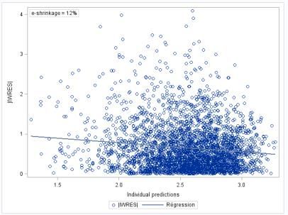
Rapport de stage                                                      CHU de Nice, Service Néphrologie

                               Remerciements

Je tiens à remercier mes enseignants ainsi que toute l’équipe au sein de laquelle j’ai travaillé, et sans
                           qui ce travail n’aurait pas été rendu possible.

   Je remercie particulièrement ma professeur Madame Christine Malot et mon maître de stage
                     Docteur Olivier Moranne pour leur précieux encadrement.

      1
Imen BOUHLEL                              Master 2 IM, Université de Nice Sophia-Antipolis, 2012/2013
Rapport de stage                                                                                        CHU de Nice, Service Néphrologie

Plan
Table of figures ........................................................................................................................................ 3
Introduction (français):............................................................................................................................ 5
Introduction:............................................................................................................................................ 6
1.     Presentation .................................................................................................................................... 7
     1.1       The Kidney Disease .................................................................................................................. 7
     1.2       The linear mixed model ........................................................................................................... 9
       1.2.1          The two-Stage Analysis.................................................................................................... 9
       1.2.2          Model ............................................................................................................................ 10
       1.2.3          Estimation...................................................................................................................... 11
       1.2.4          Empirical Bayes Estimates ............................................................................................. 12
       1.2.5          A limitation of the model: The Shrinkage ...................................................................... 13
     1.3       Discussion about the hypothesis application ........................................................................ 15
       1.3.1          State of the art .............................................................................................................. 15
       1.3.2          Focus on homoscedasticity assumption ........................................................................ 16
2.     Heteroscedasticity treatment under the linear mixed model ...................................................... 19
     2.1       Diagnosis................................................................................................................................ 19
       2.1.1          Graphical diagnoses....................................................................................................... 20
       2.1.2          Theoretical tests ............................................................................................................ 22
     2.2       Consequences of shrinkage on the validity of the diagnoses ............................................... 22
       Remark: ......................................................................................................................................... 27
     2.3       Correction .............................................................................................................................. 27
       2.3.1          Modeling heteroscedasticity ......................................................................................... 27
       2.3.2          Dependent variable transformation.............................................................................. 29
3.     Application and Results ................................................................................................................. 31
     3.1       PSPA....................................................................................................................................... 31
       3.1.1          The data set ................................................................................................................... 31
       3.1.2          Model ............................................................................................................................ 33
       3.1.3          Diagnoses....................................................................................................................... 42
       3.1.4          Treatment ...................................................................................................................... 46
       3.1.5          Results comparison ....................................................................................................... 59
4.     Discussion and Conclusion ............................................................................................................ 64
References ............................................................................................................................................. 65
Appendices ............................................................................................................................................ 67

           2
Imen BOUHLEL                                                   Master 2 IM, Université de Nice Sophia-Antipolis, 2012/2013
Rapport de stage CHU de Nice, Service Néphrologie
Table of figures
Figure 1: Proposed revised chronic kindney disease classification CKD Classification (KDIGO 2009) [A
Levey et al. Kidney International 2011]................................................................................................... 7
Figure 2: Conceptual model of CKD to organize action plan. This diagram presents the continuum of
development, progression, and complications of chronic kidney disease. Green circles represent
stages of chronic disease; aqua circles represent potential antecedents, lavender circles represent
consequences, and thick arrows betweek ellises represent risk factors associated with development,
progression, and remission of chronic kidney disease. ‘Complications’ refers to decreased glomerular
filtration rate (GFR) and cardiovascular disease. .................................................................................... 8
Figure 3: Natural history of GFR in CKD................................................................................................... 8
Figure 4 : True residuals and Shrunk residuals ...................................................................................... 14
Figure 5: Homoscedasticity situation Gujarati: Basic Econometrics, Fourth Edition, 2004] ................ 16
Figure 6: Heteroscedasticity situation [Gujarati: Basic Econometrics, Fourth Edition, 2004] .............. 17
Figure 7: Household consumption spending as function of permanent income according to Keynes 17
Figure 8: Residuals Versus individual predicted values plot presenting a cone shape ......................... 20
Figure 9 : IWRES distribution by degree of information of the data ..................................................... 22
Figure 10 : Histogram (range [-5,5]) of 1000 random intercepts drawn from the normal mixture ½ N(-
2, 1) + ½ N(2, 1). .................................................................................................................................... 23
Figure 11 : Histogram (range [-5, 5]) of the EBE of the random intercepts shown in previous figure,
calculated under the assumption that the random effects are normally distributed .......................... 24
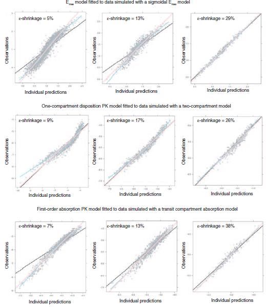
Figure 12 : Observations versus individual predictions for three different structural model
misspecifications at varying degrees of information in data, expressed through the ε-shrinkage value.
Emax, maximum drug effect; PK, pharmacokinetics ............................................................................... 25
Figure 13 : |IWRES| versus individual predictions at different degrees of shrinkage .......................... 26
Figure 14 : Power of individual weighted residual (|IWRES|) versus individual prediction (IPRED) to
detect residual model misspecification. In absence of shrinkage, the regression line of
|IWRES| versus IPRED clearly indicates residual model misspecification (left panel). With increased
shrinkage, the slope of the regression line is diminishing (right panel) ............................................... 27
Figure 15: Available covariance structures for the matrix Σi in SAS...................................................... 28
Figure 16: Influence diagnostics before and after suppressing the influent observations ................... 36
Figure 17: Summary of the population study preparation steps .......................................................... 38
Figure 18: Histogram and boxplot of number of measurements by patient ........................................ 38
Figure 19: Histogram and boxplot of time interval between consecutive measurements................... 39
Figure 20: Histogram of GFR at baseline ............................................................................................... 39
Figure 21: Boxplot of GFR at baseline ................................................................................................... 40
Figure 22: QQ plot of Cholesky residuals .............................................................................................. 40
Figure 23: Histograms of the random effects ....................................................................................... 41
Figure 24: Observations versus individual predicted values ................................................................. 41
Figure 25: Residuals versus (individual) predicted values ..................................................................... 42
Figure 26: Absolute residuals versus (individual) predicted values ...................................................... 42
3
Imen BOUHLEL Master 2 IM, Université de Nice Sophia-Antipolis, 2012/2013
Rapport de stage                                                                                      CHU de Nice, Service Néphrologie

Figure 27: Student Residuals versus time ............................................................................................. 43
Figure 28: |IWRES| versus individual predictions ................................................................................. 43
Figure 29: IWRES versus time ................................................................................................................ 44
Figure 30: Absolute IWRES versus individual predictions slope evolution with shrinkage level .......... 45
Figure 31: IWRES versus time slope evolution with shrinkage level ..................................................... 45
Figure 32: Absolute IWRES versus individual prediction for model fitted to the 90th percentile of total
number of measurements by patient ................................................................................................... 45
Figure 33: IWRS versus time slope for model fitted to the 90th percentile of total number of
measurements by patient ..................................................................................................................... 46
Figure 34: GFR variance versus GFR mean ............................................................................................ 47
Figure 35: Information criteria comparison between model M1 and model M2 ................................. 50
Figure 36: Logarithm, Square root, Cube root and Fourth root functions ............................................ 51
Figure 37: Residuals versus individual predictions for models M1, M3, M4, M5 and M6 .................... 52
Figure 38: Absolute residuals versus individual predictions for models M1, M3, M4, M5 and M6 ..... 53
Figure 39: Absolute IWRES versus individual predictions slope evolution by degree of shrinkage for
model M3 .............................................................................................................................................. 54
Figure 40: Absolute IWRES versus individual predictions slope evolution by degree of shrinkage of the
data for the different transformed models ........................................................................................... 55
Figure 41: QQ plot of the Cholesky residuals for the different models ................................................ 56
Figure 42: Random effects distribution for the different models ......................................................... 57
Figure 43: Observations versus individual predictions for the different models .................................. 58

         4
Imen BOUHLEL                                                  Master 2 IM, Université de Nice Sophia-Antipolis, 2012/2013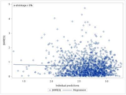
Rapport de stage                                                      CHU de Nice, Service Néphrologie

     Introduction (français):
Le modèle linéaire simple repose sur plusieurs hypothèses qui sont l’exogénéité des variables
explicatives, l’indépendance des variables explicatives, la normalité des résidus, l’homoscédasticité
des résidus, et l’absence d’autocorrélation des résidus.

 En particulier, la plupart des résultats obtenus jusqu’à aujourd’hui à partir des différents modèles de
régression des variables quantitatives sont basés sur l’hypothèse d’homoscédasticité des résidus.
Cependant, cette hypothèse est rarement vérifiée en pratique. C’est principalement le cas lorsqu’on
étudie les séries temporelles ou les données longitudinales (spécialement les données biologiques,
par exemple lors de suivis de maladies évolutives ou de réponses aux traitements) car elles sont plus
complexes à évaluer.

L’hétéroscédasticité est définie comme la non-homoscédasticité, ce qui veut dire la non-constance
des erreurs ou résidus. En d’autres mots, on observe de l’hétéroscédasticité lorsque les résidus
dépendent de l’observation ou du temps. Ce phénomène peut généralement être secondaire à des
valeurs aberrantes, une mauvaise spécification ou adéquation du modèle, une mauvaise
transformation des données ou une asymétrie des variables dépendantes

La violation de l’hypothèse d’homoscédasticité peut remettre en question la validité de la
modélisation, des estimations et des résultats des tests statistiques usuels. Néanmoins, il est facile de
contourner ce problème dans le cadre du modèle linéaire simple et lorsque la fonction scédastique
est complétement ou partiellement connue. En effet, il est possible de tester la présence
d’hétéroscédasticité, et d’utiliser des estimateurs transformés robustes. Par contre, pour des
modèles plus complexes, comme le modèle linéaire mixte, la littérature reste relativement pauvre
sur ce sujet.

En sciences appliquées biomédicales, nous sommes souvent confrontés à des collections de données
corrélées, répétées souvent déséquilibrées. Ce terme générique regroupe une multitude de
structures de données, telles que les observations multi variées, les « clustured data », les mesures
répétées et les données longitudinales. Le modèle linéaire simple n’est pas adapté à ce type de
structures de données car il ne prend pas en compte le caractère « spécifique au sujet » des
données. En conséquence, des modèles plus complexes sont développés. Nous choisissons de nous
intéresser au modèle linéaire mixte, qui est largement utilisé pour traiter les données longitudinales
répétées déséquilibrées particulièrement adaptées à la modélisation des pathologiques chroniques
en recherche biomédicale.

L’objectif de mon travail est d’étudier les diagnostics de l’hétéroscedasticité proposés dans le cadre
du modèle linéaire mixte, d’étudier les effets potentiels de la non-prise en compte de
l’hétéroscédasticité dans la modélisation longitudinale de données quantitatives à partir de données
réelles (modélisation évolution maladie rénale chronique), et de proposer des méthodes corrections.

Ce travail présente en première partie le terrain du stage, à savoir la maladie rénale chronique (MRC)
puis le modèle linéaire mixte ainsi que la justification de son choix pour modéliser l’évolution de la
MRC en recherche biomédicale. La deuxième partie traite du diagnostic de l’hétéroscédasticité sous
le modèle linéaire mixte ainsi que les corrections proposées. Dans la dernière partie, les résultats
seront appliqués à un jeu de données réelles dans le cadre d’une étude observationnelle de
l’évolution de la maladie rénale chronique qui seront analysés à l’aide du logiciel SAS.

      5
Imen BOUHLEL                              Master 2 IM, Université de Nice Sophia-Antipolis, 2012/2013
Rapport de stage                                                     CHU de Nice, Service Néphrologie

     Introduction:

   The linear mixed model relies on multiple assumptions that are the exogeneity of the explicative
   covariables, the independency of the explicative covariables, the residuals normality, the residual
   homoscedasticity and the non-autocorrelation of the residuals.

   In particular, most of the results obtained up to now from the different regression models of
   quantitative variables are based on the assumption of homoscedasticity of errors. However, such
   a strong assumption is rarely verified in practice. It is principally the case when studying time
   series or longitudinal data (especially biological data, for example when monitoring progressive
   disease or treatment response) because they are more complex to evaluate.

   The heteroscedasticty is defined by the non-homoscedasticity, which means non-constancy of
   the errors or residuals. In other words, there is heteroscedasticity when errors depend on the
   observation or on time. This phenomenon may be secondary to outliers, model misspecification,
   bad data transformation or asymmetry of the dependent variables.

   The violation of the assumption of homoscedasticity can call into question the model validity,
   parameters estimations and usual statistical tests validity. Nevertheless, it is easy to get around
   this problem under the linear simple model and when the scedastic function is completely or
   partially known. In fact, it is possible to test the presence of heteroscedasticity, and to use robust
   transformed estimators. However, for some more complex models such as the linear mixed
   model, literature is still relatively poor about this subject.

   In applied biomedical sciences, one is often confronted with the collection of a correlated
   repeated and often unbalanced data. This generic term embraces a multitude of data structures,
   such as multivariate observations, clustered data, repeated measurements and longitudinal data.
   The linear simple model is not adapted to these data structures because it does not take into
   account the “subject-specific” trait of the data. In consequence, more complex models are
   developed. We chose to focus on the linear mixed model, which is widely used for the study of
   longitudinal continuous repeated and unbalanced data, particularly adapted to the modelisation
   of chronic disease in biomedical research.

   This works presents in the first section generalities about the chronic kidney disease and the
   linear mixed model, as well as the justification of its choice for modeling the chronic kidney
   disease in biomedical research. The second section treats of heteroscedasticity diagnostics under
   the linear mixed model and proposes corrections. In the third sections, results are applied to a
   real dataset of an observational study describing the evolution of the chronic kidney disease
   which will be analyzed using SAS software.

      6
Imen BOUHLEL                             Master 2 IM, Université de Nice Sophia-Antipolis, 2012/2013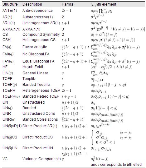
Rapport de stage                                                                    CHU de Nice, Service Néphrologie

1.         Presentation

        1.1       The Kidney Disease

Chronic kidney disease (CKD) was defined based on the presence of kidney damage or glomerular
filtration rate (GFR < 60 ml/min per 1.73m2) for more than 3 months.

CKD is a concept and was classified in several prognosis stages based on the level of GFR, albuminuria
and clinical diagnosis to help action plan (Figure 1, 2).

The GFR defines the renal function and can be estimated with a formula using the dosage of
creatinine in blood corrected by age, sex and ethnicity. The more usual formula is called MDRD
formula:

GFR (ml/min/1.73m²)=186 x creatinine (mg/dl)-1,154 x age-0,203 x 0,742 (for women) x 1,21 (for Afro-
Americans).

Where age is expressed in years.

CKD is an evolutive disease with rate of decline of GFR usually consider as linear (slope). GFR decline
is variable based on the underlying population, cause of CKD, presence of albuminuria/proteinuria,
comorbidities and age. The conceptual model of CDK is presented figure 2 and the natural history of
the evolution of CKD is presented figure 3.

The importance of determining the rate of decline in kidney function (slope) over time is to identify
individuals who are progressing at a more rapid rate than normal again and to predict the final stage
of CDK which needs special treatment such as dialysis to maintain life, and because a higher slope is
associated with increased morbidity and mortality. Finally, individuals who are ‘‘rapid progressors’’
should be targeted to slow their progression with specific treatment and to prevent adverse
outcomes.

Clinical Diagnosis                GFR stages (ml/min per 1,73 m²        Albuminuria stages (ACR, mg/g)
Diabetes                                         > 90                                 < 30
Hypertension                                   60 - 89
Glomerular disease                             45 - 59                              30 - 299
Many others                                    30 - 44
Transplant                                     15 - 29                               > 300
Unknown                                          < 15
Abreviations : ACR, albumin-to-creatinine ratio ; GFR, glomerular filtration rate; KDIGO, Kidney
Disease: Improving Global Outcomes.

    Figure 1: Proposed revised chronic kindney disease classification CKD Classification (KDIGO 2009) [A Levey et al. Kidney
                                                                         1
                                                     International 2011]

1
    Levey and al, Kidney International 2011, The definition, classification, and prognosis of chronic kidney

          7
Imen BOUHLEL                                        Master 2 IM, Université de Nice Sophia-Antipolis, 2012/2013
Rapport de stage                                                                    CHU de Nice, Service Néphrologie

Figure 2: Conceptual model of CKD to organize action plan. This diagram presents the continuum of development,
progression, and complications of chronic kidney disease. Green circles represent stages of chronic disease; aqua circles
represent potential antecedents, lavender circles represent consequences, and thick arrows betweek ellises represent
risk factors associated with development, progression, and remission of chronic kidney disease. ‘Complications’ refers to
decreased glomerular filtration rate (GFR) and cardiovascular disease.

                                         Figure 3: Natural history of GFR in CKD.

       8
Imen BOUHLEL                                    Master 2 IM, Université de Nice Sophia-Antipolis, 2012/2013
Rapport de stage                                                     CHU de Nice, Service Néphrologie

    1.2      The linear mixed model
         1.2.1 The two-Stage Analysis
Longitudinal data are often composed of repeated data within each subject. Thus, longitudinal data
has a hierarchical structure introducing correlations for the observations within a subject. As a
consequence, it would not be adequate to analyze this type of structure through a simple linear
model which does not take into account the subject-specific trait of the data.

Moreover, in practice, longitudinal data are rarely balanced in the sense that the number of
measurements for each subject is rarely the same and/or that measurements are not taken at fixed
time points.This type of datasets are called unbalanced datasets. Thus, many longitudinal datasets
cannot be analyzed using multivariate regression techniques.

As an alternative, the linear mixed model is particularly adapted to this type of datasets (unbalanced
datasets). In fact, the linear mixed model arises from a “two-stage analysis”. The main idea of the
“two-stage analysis” is that subject-specific longitudinal profiles can be approximated by simple
linear regression functions in the first stage, and the estimates can be related to known covariates as
treatment or disease in the second one. The general linear mixed model is then the result of
combining the two stages into one statistical model, containing less estimations parameters, and
then considered as a more parsimonious model.

             1.2.1.1    Stage 1
Let the random variable Yij denote the (possibly transformed) response of interest, for the ith
individual, measured at time tij, i=1,…,N, j=1,…,ni, and let Yi be the ni-dimensional vector of all
repeated measurements for the ith subject, that is, Yi = ( Yi1, Yi2, … , Yini)’. The first stage of the
two-stage approach assumes that Yi satisfies the linear regression model

                                    Yi = Zi βi +εi                                              (1.1)

where Zi is a (ni x q) matrix of known covariates, modeling how the response evolves over time
for the ith subject. Further, βi is a q-dimensional vector of unknown subject-specific regression
coefficients, and εi is a vector of residual components εij, j=1,…,ni. It is usually assumed that all εi
are independents and normally distributed with mean vector zero, and covariance matrix σ²I ni,
where Ini is the ni-dimensional identity matrix.

              1.2.1.2     Stage 2
In a second step, a multivariate regression model of the form

                                   βi = Ki β + bi                                              (1.2)

is used to explain the observed variability between the subjects, with respect to their subject-
specific regression coefficients βi. Ki is a (q x p) matrix of known covariates, and β is a p-
dimensional vector of unknown regression parameters. Finally, the bi are assumed to be
independent, following a q-dimensional normal distribution with mean vector zero and general
covariance matrix D.
      9
Imen BOUHLEL                              Master 2 IM, Université de Nice Sophia-Antipolis, 2012/2013
Rapport de stage CHU de Nice, Service Néphrologie
1.2.1.3 Two-Stage Analysis
First, all βi are estimated by fitting model (1.1) to the observed data vector yi of each subject
separately, yielding estimates βi*.Hereafter, model (1.2) is fitted to the estimates βi*, providing
inferences for β.
Nevertheless, the two-stage analysis suffers from at least two problems. First, information is lost
in summarizing the vector yi of observed measurements for the ith subject by βi*. Second,
random variability is introduced by replacing the βi in model (1.2) by their estimates βi*.
Moreover, the covariance matrix of βi* highly depends on the number of measurements available
for the ith subject as well as on the time points at which these measurements were taken, and
this has not been taken into account in the second stage of the analysis.
These problems can be solved by combining the two stages into one model, the so-called linear
mixed model (or the linear mixed-effects model).
1.2.2 Model
1.2.2.1 Model and Assumptions
In order to combine the models from the two-stage analysis, we replace βi in (1.1) by expression
(1.2), yielding
Yi = Xi β + Zi bi + εi (1.3)
where Xi = ZiKi is the appropriate (ni x p) matrix of unknown covariates, and where all other
components are as defined earlier. Model (1.3) is called a linear mixed (-effects) model with
fixed effects β and with subject-specific effects bi. It assumes that the vector of repeated
measurements on each subject follows a linear regression model where some of the regression
parameters are population-specific. The bi are assumed to be random and are therefore often
called random effects.
In general, a linear mixed model is any model which satisfies (Laird and Ware 1982)2
Yi = Xi β + Zi bi + εi (1.4)
bi ~ N(0, D),
εi ~ N(0,Σi),
b1,…,bN, ε1,…, εN independant,
where Yi is the ni-dimensional response vector for subject i, 1≤ i ≤ N, N is the number of subjects,
Xi and Zi are (ni x p) and (ni x q) dimensional matrices of known covariates, β is a p-dimensional
vector containing the random effects, and εi is an ni-dimensional vector of residual components.
Finally, D is a general (q x q) covariance matrix with (i, j) element dij = dji and Σi is (ni x ni)
covariance matrix which depends on i only through its dimension ni, i.e. the set of unknown
parameters in Σi will not depend upon i(homoscedasticity assumption).
2
Laird and Ware (1982), Random effects models for longitudinal data.
10
Imen BOUHLEL Master 2 IM, Université de Nice Sophia-Antipolis, 2012/2013Rapport de stage CHU de Nice, Service Néphrologie
It follows from (1.4) that, conditional on the random effect bi, Yi is normally distributed with
mean vector Xi β + Zi bi and with covariance matrix Σi. Further, bi is assumed to be normally
distributed with mean vector 0 and covariance matrix D. Let f(yi |bi) and f(bi) be the
corresponding density functions. The marginal density function of Yi is then given by
f(yi) = ∫ f(yi|bi) f(bi) dbi (1.5)
which can be shown to be the density function of an ni-dimensional normal distribution with
mean vector Xi β and with covariance matrix Vi = ZiDZi’ + Σi.
Yi ~ N(Xi β, Vi = ZiDZi’ + Σi ) (1.6)
1.2.3 Estimation
Inference is based on the marginal distribution for the response Yi :
Yi ~ N(Xi β, Vi = ZiDZi’ + Σi )
Let α denote the vector of all variance and covariance parameters (usually called variance
components) found in Vi = ZiDZi’ + Σi , that is, α consists of the q(q+1)/2 different elements of D
and of all parameters in Σi. Finally, let θ = (β’, α’)’ be the s-dimensional vector of all parameters in
the marginal model for Yi.
The classical approach to inference is based on estimators obtained from maximizing the
marginal likelihood function:
LML = ∏i=1N { (2π)-ni/2 |Vi(α)|-1/2 exp(-1/2 (Yi – Xiβ)’ Vi-1(α) (Yi –Xiβ)) } (1.7)
with respect to θ.
1.2.3.1 Estimation of β
Let us first assume α to be unknown. The maximum likelihood estimator (MLE) of β, obtained
from maximizing (1.7), conditional on α, is then given by (Laird and Ware 1982)3
β*(α) = ( ∑i=1N Xi’WiXi)-1 ∑i=1N Xi’Wiyi (1.8)
where Wi = Vi-1.
1.2.3.2 Estimation of the variance components
When α is not known, but an estimate α* is available, we can set Vi* = Vi(α*) = Wi-1*, and estimate
β by using the expression (1.8) in which Wi is replaced by Wi*. Two frequently used methods for
estimating α are maximum likelihood estimation and restricted maximum likelihood estimation.
The maximum likelihood estimator (MLE) of α is obtained by maximizing (1.7) with respect to α,
after β is replaced by (1.8). This approach arises naturally when we consider the estimation of β
and α simultaneously by maximizing the joint likelihood (1.7)
3
Laird and Ware (1982), Random effects models for longitudinal data.
11
Imen BOUHLEL Master 2 IM, Université de Nice Sophia-Antipolis, 2012/2013Rapport de stage CHU de Nice, Service Néphrologie
The ML estimates of the covariance parameters are biased, because they do not take into
account the loss of freedom degrees induced by the estimation of the fixed effects. To correct this
bias, we can estimate the parameters by restricted maximum likelihood (REML) estimation.
The REML estimation is obtained from maximizing the likelihood function of a set of error
contrasts U= A’Y where A is any (n x (n-p)) full-rank matrix with columns orthogonal to the
columns of the X matrix. The vector U then follows a normal distribution with mean zero and
covariance matrix A’V(α)A, which is not dependent on β any longer.
The so-called REML likelihood function to maximize is then:
LREML (θ) = |∑i=1N XiWi(α)Xi|-1/2 LML(θ) (1.9)
1.2.3.3 Estimation of Var(β *)
We saw that the vector β of fixed effects is estimated by (1.8):
β*(α) = ( ∑i=1N Xi’WiXi)-1 ∑i=1N Xi’Wiyi
in which the unknown vector α of variance components is replaced by its Maximum Likelihood
(ML) or (REML) estimate.
Under the marginal model (1.6), and conditionally on α, β*(α) follows a multivariate
distribution with mean vector β and with variance-covariance matrix:
Var(β*) = ( ∑i=1N Xi’WiXi)-1 ( ∑i=1N Xi’Wi V(Yi)Wi Xi) (∑i=1N Xi’WiXi)-1 (1.10)
Where Wi = Vi-1(α).
1.2.4 Empirical Bayes Estimates
1.2.4.1 Estimation
Since the random effects in model (1.4) are assumed to be random variables, they are estimated
using Bayesian techniques (see, for example, Box and Tiao 19924 or Gelman al. 19955). As discussed
in Section 1.2.1, the distribution of the vector Yi of responses for the ith individual, conditional on
that individual’s specific regression coefficients bi, is multivariate normal with mean vector Xiβ + Zibi
and with covariance matrix ∑i . Further, the marginal distribution of bi is multivariate normal with
mean vector 0 and covariance matrix D. In the Bayesian literature, this last distribution is usually
called the prior distribution of the parameters bi since it does not depend on the data Yi. Once
observed values yi for Yi have been collected, the so-called posterior distribution of bi, defined as the
distribution of bi, conditional on Yi=yi, can be calculated. If we denote the density function of Yi
conditional on bi, and the prior density function of bi by f(yi|bi) and f(bi), respectively, we have that
the posterior density function of bi given Yi=yi is given by (dependence on certain components of θ is
suppressed):
f(bi |yi) = f(bi | Yi=yi) = f(yi|bi) f(bi) / ∫ f(yi|bi) f(bi) dbi (1.11)
4
Box and Tiao (1992), Bayesian inference in statistical analysis.
5
Gelman and al (1995), Bayesian data analysis.
12
Imen BOUHLEL Master 2 IM, Université de Nice Sophia-Antipolis, 2012/2013Rapport de stage CHU de Nice, Service Néphrologie
Using the theory on general Bayesian linear models (Smith 19736, Lindley and Smith 19727), it can be
shown that (1.11) is the density of a multivariate normal distribution. Very often, bi is estimated by
the mean of this posterior distribution, called the posterior mean of bi. This estimate id then given
by:
bi*(θ) = E [bi | Yi=yi ]
= ∫ bi f(bi|yi) dbi
= D Zi’Wi(α) (yi – Xiβ) (1.12)
The resulting estimates for the random effects are called “Empirical Bayes Estimates” (EBE).
1.2.4.2 Var(bi*(θ))
The covariance matrix of bi*(θ) is (Laird and Ware 1982)8:
Var(bi*(θ)) = D Zi’ { Wi - Wi Xi ( ∑i=1N Xi’WiXi) -1 Xi’Wi } ZiD (1.13)
Where Wi = Vi-1(α).
Yet, (1.13) underestimates the variability in bi*(θ) - bi since it ignores the variation of bi. Therefore,
inference for bi is usually based on
Var ( bi*(θ) – bi ) = D – Var(bi*(θ)) (1.14)
as an estimator for the variation in bi*(θ) – bi (Laird and Ware 1982)9.
1.2.5 A limitation of the model: The Shrinkage
1.2.5.1 η-Shrinkage
The Empirical Bayes Estimates (EBE) are examples of shrinkage estimators.
In fact, let us replace bi* by (1.12) in the following expression:
Yi* = Xiβ*+ Zibi*
= Xiβ* + ZiDZi’Vi-1 (yi- Xiβ*)
= (Ini – ZiDZi’Vi-1) Xiβ*+ ZiDZi’Vi-1 yi
=∑i Vi-1 Xiβ* + (Ini - ∑i Vi-1) yi (1.15)
We see then that the prediction of the response for the subject i can be interpreted as a weighted
average of the population mean Xiβ* and the observed data yi. The average profile is weighted by
6
Smith (1973), A general Bayesian linear model.
7
Lindley and Smith (1972), Bayes estimates for the linear model.
89
, Laird and Ware (1982), Random effects models for longitudinal data.
13
Imen BOUHLEL Master 2 IM, Université de Nice Sophia-Antipolis, 2012/2013Rapport de stage CHU de Nice, Service Néphrologie
(∑iVi-1), while the observed data is weighted by (Ini - ∑i Vi-1). (∑i Vi-1) is in fact the “quotient” of residual
covariance matrix ∑I and the overall covariance matrix. Thus, larger weights are given to the average
profile if the residual variability (∑i) is larger than the between subject variability (ZiDZi’). This is called
the “shrinkage” phenomenon: the EBE “shrink” toward zero, and then the individual prediction
“shrink” toward the population mean which is Xiβ.
This phenomenon of shrinkage was referred to in the Bayesian literature (Carlin and Louis 199610,
Strenio, Weisberg, and Bryk 198311).
Measures have in consequence been introduced in order to evaluate the amplitude of the shrinkage.
Earlier, we introduced an estimator for the variation in bi*(θ) – bi :
Var (bi*(θ) – bi ) = D – Var(bi*(θ))
This implies that for any linear combination λ of the random effects,
Var (λ‘ bi*) ≤ Var (λ‘ bi )
In consequence,
Var (bi*) ≤ Var (bi)
As a result, an estimator of the shrinkage of the random effects would be:
η-shrinkage= 1 – (Var (bi*)/ Var (bi)) (1.16)
1.2.5.2 ε-Shrinkage
Similarly, we can observe shrinkage of the residuals, which means that the residuals “shrink” toward
zero.
Figure 4 : True residuals and Shrunk residuals
10
Carlin and Louis (1996), Bayes and empirical bayes methods for data analysis.
11
Strenio, Weisberg, and Bryk (1983), Empirical bayes estimatation of individual growth-curve
parameters and their relationship to covariates.
14
Imen BOUHLEL Master 2 IM, Université de Nice Sophia-Antipolis, 2012/2013Rapport de stage CHU de Nice, Service Néphrologie
In practice, we will have:
Var(εij )1/2≤ σε (1.17)
Where Var(εij )1/2 is the Residuals standard deviation given by the data, and σε is the residuals
standard deviation given by the residual error model.
We know that (εij / Var(εij )1/2 has standard deviation equal to one, since residuals are assumed to
have a normal distribution, and (εij/ Var(εij )1/2) represent the standardized residuals.
Let be the Individual Weighted Residuals:
IWRES = εij / σε (1.18)
Given (1.17), we can deduce that IWRES have standard deviation inferior to 1. Hence, a measure of
the residuals shrinkage can be deduced:
ε-shrinkage = 1 – SD (IWRES) (1.19)
The consequences of the presence of shrinkage in the data will be discussed later in the second
section.
1.3 Discussion about the hypothesis application
1.3.1 State of the art12
To remind, the key assumptions of the linear mixed model are:
- Normality of the random effects distribution;
- Independency of the response given the random effects i.e. independency of the errors;
- Normality of the error;
- Homoscedasticity of the error.
Concerning the first assumption, several studies have shown that maximum likelihood inference on
fixed effects is robust to non-gaussian random effects distribution (Butler and Louis, 199213; Verbeke
and Lesaffre, 199714; Zhang and Davidian, 200115).
As for the second assumption, some results suggest robustness to misspecification of the covariance
structure. First, Liang and Zeger (1986)16 have demonstrated convergence of fixed effects estimates
obtained by generalized estimating equations (GEE) whatever the working covariance matrix. Given
that, for the linear model, estimating equations obtained by derivation of the maximum likelihood
12
Jacqmin-Gadda, Sibillot, Molina and Thiébaut (2007),Robustness of the linear mixed model to
misspecified error distribution.
13
Butler and Louis (1992), Random effects models with non-parametric priors.
14
Verbeke and Lesaffre (1997), The effect of misspecifying the random effects distribution in linear
mixed models for longitudinal data.
15
Zhang and Davidian (2001), Linear mixed models with flexible distributions of random effects for
longitudinal data.
16
Liang and Zeger (1986), Longitudinal data analysis using generalized linear models.
15
Imen BOUHLEL Master 2 IM, Université de Nice Sophia-Antipolis, 2012/2013Rapport de stage CHU de Nice, Service Néphrologie
are identical (except for the covariance estimator) to GEE with appropriate covariance structure, this
result demonstrates convergence of maximum likelihood estimator for fixed effects in the linear
mixed model when the covariance structure is not correct. On the other hand, Liang and Zeger
(1986)17 demonstrated that variance estimates of fixed effects may be biased when the covariance
structure is not correct and they recommend the use of the robust sandwich estimate (Royall,
1986)18. However, this robust estimate may be unstable for small sample sizes.
However, the two last assumptions, normality and homoscedasticity of the error, have been less
studied.
1.3.2 Focus on homoscedasticity assumption
1.3.2.1 Heteroscedasticity under the linear simple model
Homoscedasticity is one of the assumptions of the simple model.
We say that there is heteroscedasticity when
V( ε| X) ≠ σ² I
Illustration:
Figure 5: Homoscedasticity situation Gujarati: Basic Econometrics, Fourth Edition, 2004]
17
Liang and Zeger (1986), Longitudinal data analysis using generalized linear models.
18
Royall (1986), Model robust confidence intervals using maximum likelihood estimators.
16
Imen BOUHLEL Master 2 IM, Université de Nice Sophia-Antipolis, 2012/2013Rapport de stage CHU de Nice, Service Néphrologie
Figure 6: Heteroscedasticity situation [Gujarati: Basic Econometrics, Fourth Edition, 2004]
Example of Cross-sectional data: Keynes’s Consumption theory:
One of his main features is that the marginal propensity to consume (MCP) falls with income. In fact,
as we can see in the following graph, for two different categories of households (say wealthy
households and less wealthy ones), the slope is not the same. This illustrates that different categories
of households have different behaviors. In particular, knowing that the permanent income is
partitioned between consumption and saving, we deduce that the wealthier households will save a
more important part of their income that the less wealthy households will do. In consequence, the
variation of the saving of the less wealthy households will be less important than the variation of the
saving of the wealthier households. Thus, when treating cross-sectional data of households’ saving
for example, it is evident that we will observe heteroscedasticity.
Figure 7: Household consumption spending as function of permanent income according to Keynes
17
Imen BOUHLEL Master 2 IM, Université de Nice Sophia-Antipolis, 2012/2013Rapport de stage CHU de Nice, Service Néphrologie
1.3.2.1.1 Consequences
If the homoscedasticity assumption is respected, the OLS estimators are convergent and BLUE (Best
Linear Unbiased Estimator). An estimator is said to be BLUE if it is:
- It is linear, that is, a linear function of a random variable, such as the dependent variable in
the regression model.
- It is unbiased, that is, the average or expected value of the estimator is equal to the true
value.
- It has minimum variance in the class of all such linear unbiased estimators; an unbiased
estimator with the least variance is known as an efficient estimator.
1.3.2.1.1.1Ordinary Least Squares (OLS) estimator still unbiased and
convergent
When we have heteroscedasticity, the OLS estimator is still unbiased and convergent. In fact, we
do not use the hetescedasticity assumption to prove that the estimator is unbiased. Only H1, H2
and H3 are used.
1.3.2.1.1.2 BLUE?
But OLS estimator is not Best Linear Unbiased Estimator (BLUE) anymore. In fact, it is no longer
efficient:
V[β*|X] = E [(X’X)-1 X’εε’X (X’X)-1 | X] > V[β*|X] = σ² (X’X)-1
1.3.2.1.1.3 Student and Fisher tests
In consequence, we cannot anymore apply the usual statistical tests (Student, Fisher). In fact,
these tests assume that the variance of the coefficient is equal to:
V[β*|X] = σ² (X’X)-1
Which is not true anymore.
1.3.2.1.2 Treatment
1.3.2.1.2.1 Diagnosis
The literature about the detection of heteroscedasticity under the simple model is very rich. In fact,
there exist graphical methods as well as statistical tests.
The principal graphical diagnosis is plotting the residuals against the predicted value (of the
dependent variable). The plotted residuals should not have a particular form. If they do, then
there is certainly heteroscedasticity over the observations.
The main statistical tests are Golfred Quant test (1965), Breush Pagan test (1979)19, White test
(1980)20 and Gleisjer test (1969).
19
Breausch and Pagan (1979), A simple test for heteroscedasticity and random coefficient variation.
18
Imen BOUHLEL Master 2 IM, Université de Nice Sophia-Antipolis, 2012/2013Rapport de stage CHU de Nice, Service Néphrologie
1.3.2.1.2.2 Correction
The literature about the correction of heteroscedasticity is also rich. The main methods are White’s
Robust Standard Errors (White, 1980)21 and the Feasible General Least Squares (where we use a
general form of the scedastic function that is V(ε|X) = σ² exp(δ0 + δ1 X1 + … + δk Xk)) . Another widely
used method is transforming the depending variable.
1.3.2.2 Heteroscedasticity under the linear mixed model
Heteroscedasticity is also one of the key assumptions of the linear mixed (Laird and Ware 1982)22.
But unlike for the (linear) simple model, consequences of misspecifying assumptions of the linear
mixed model still are not well known since the literature is still relatively poor.
The homoscedasticity assumption under the linear mixed model writes:
εi ~ N(0, σ² Ini ) (1.15)
The variance-covariance matrix of the residual has then the following form:
σ² 0 … 0
0 σ² 0 … 0
.
Σi = .
.
0 … 0 σ²
2. Heteroscedasticity treatment under the linear mixed model
2.1 Diagnosis
Let us first define the different types of residuals under the linear mixed model.
Since there exist different types of predictions in the linear mixed model, we can define different
types of residuals: The marginal residuals Yi - Xiβ* with variance Vi – Xi(Σi=1k Xi’Vi-1 Xi’)-1 Xi , and the
subject-specific residuals or conditional residuals εi* = Yi - Xiβ* - Zibi* . By replacing bi by the
empirical bayes estimates (or BLUP: Best Linear Unbiased Predictor) (see (1.12)), we obtain
20
White (1980), A heteroskedasticity-consistent covariance matrix estimator and a direct test for
heteroskedasticity.
21
White (1980), A heteroskedasticity-consistent covariance matrix estimator and a direct test for
heteroskedasticity.
22
Laird and Ware (1982), Random effects models for longitudinal data.
19
Imen BOUHLEL Master 2 IM, Université de Nice Sophia-Antipolis, 2012/2013Rapport de stage CHU de Nice, Service Néphrologie
εi* = Yi - Xiβ* - Zibi*
= Yi - Xiβ* - Zi D Zi’Vi-1 (Yi – Xiβ*)
= (Ini - Zi D Zi’Vi-1 ) (Yi – Xiβ*)
= Σi Vi-1 (Yi – Xiβ*)
And Var (εi*) = Σi Vi-1 Var (Yi – Xiβ*) Vi-1 Σi .
In consequence, we note that even under the linear mixed model where Σi = σ² Ini , the estimated
conditional residuals are correlated. In particular, their distribution depends on the choice of Vi and
on the prior distribution of the random effects.
Remark:
In the following, residuals stand for conditional residuals
2.1.1 Graphical diagnoses
The usual tests for diagnosing heteroscedasticity under the linear mixed model are principally
graphical tests:
2.1.1.1 Residuals Versus Individual predicted values
The evaluation of the assumption of constancy of the residual error variance (or homoscedasticity
assumption) is difficult under the linear mixed model since the conditional residuals εi* do not have
constant variance and are correlated. In particular, suppose the model contains one random effect,
say time. Then, Var (εi*) depends on time. However, if σ1²* tij² remains small compared to the
variance of the intercept σ0² and of the error σe², we may consider that Var (εi* ) is approximately
independent of time, and evaluate the assumption of homoscedasticity by representing εi* (the
estimated residuals) versus E(Yij | bi*) ( the individual predicted values).
The residuals should not have a particular shape. In fact, the residuals are assumed not to depend on
i or j. Consequently, they should not depend on the individual predicted values. However, the
residuals can have a particular shape. Very often, we observe that the residuals show a cone form,
which means that the residuals increase or decrease in function of the individual predicted values.
The following figure shows an example of the residuals versus individual predicted values plot,
presenting a cone shape, since the spread of the residuals increases with the individual predicted
values.
Figure 8: Residuals Versus individual predicted values plot presenting a cone shape
20
Imen BOUHLEL Master 2 IM, Université de Nice Sophia-Antipolis, 2012/2013Rapport de stage CHU de Nice, Service Néphrologie
Remark:
Another commonly used plot is the plot the absolute value of the residuals versus the individual
predicted values since it may show more clearly the possibly existent relationship between both.
2.1.1.2 Standardized residuals versus covariates
Another used graphical test is the plot of studentized residuals versus covariates, such as studentized
residuals are estimates of the standardized residuals.
The standardized residuals are defined by:
εi*/( Var(εi*)1/2 )= εi* /( vi1/2)
Where εi* is an estimation of εi and vi its variance.
And the studentized residuals are defined by:
εi* / (vi*1/2)
The justification of the use of the “standardized” residuals is that even under the homoscedasticity
assumption, the estimated residuals do not have the same variance. This is why we calculate the
standardized version in order to make them comparable.
The aim of this plot is to show whether there exists a relationship between the residuals and the
different covariates in order to eventually detect the source of heteroscedasticity. This also permits
to evaluate whether the effect of this covariate is correctly specified and to detect outliers.
2.1.1.3 Individual Weighted Residuals (IWRES) based diagnoses
Another type of residuals can also be used, which is the Individual Weighted Residuals (IWRES):
IWRES = εij / σε
Where εij are the conditional residuals and σε is the residuals standard deviation given by the residual
error model. This type of residuals will be more detailed in the section 2.2.
The principal used IWRES based diagnoses are similar to those based on the conditional residuals,
that are:
- IWRES versus Individual predicted values,
- IWRES versus covariates,
and are interpreted similarly. However, it is preferable to use the IWRES based diagnoses because
they are “shrinkage-sensitive” (see section2.2).
As will be explained in the section 2.2, results from all these diagnostics should be interpreted with
caution.
21
Imen BOUHLEL Master 2 IM, Université de Nice Sophia-Antipolis, 2012/2013Rapport de stage CHU de Nice, Service Néphrologie
2.1.2 Theoretical tests
Few theoretical tests for diagnosing heteroscedasticity under the linear mixed model exist. Among
them:
2.1.2.1 The Score test
Ahn(2000)23 proposed the score test to examine the assumption of constant variance in linear mixed
models. He stated that when heteroscedasticity occurs in linear mixed model, the variances of errors
and random effects may depend on the values of one or more of the explanatory variables or on
other relevant quantities such as time or spatial ordering. He then modeled the variance as a
function of these quantities, and developed a score test for diagnosing homoscedasticity.
2.1.2.2 The likelihood ratio test
The likelihood ratio test (for equal variances) compares a restricted model where the residual
variance σi² = σ² to an unrestricted model where a specific function is used for σi². Such a likelihood
test can be used as a robust test for a constant variance in residuals or a time series if the data is
partitioned into group24.
2.2 Consequences of shrinkage on the validity of the diagnoses
The presence of shrinkage in the data is problematic. In fact, the lower the degree of information of
the data is, the higher the shrinkage is:
Figure 9 : IWRES distribution by degree of information of the data
23
Ahn (2000), Score Test for Detecting Non-Constant Variances in Linear Mixed Models.
24
JM van Zyl (2011), The laplace likelihood ratio test for heteroscedasticity.
22
Imen BOUHLEL Master 2 IM, Université de Nice Sophia-Antipolis, 2012/2013Rapport de stage CHU de Nice, Service Néphrologie
And the higher the shrinkage is, the less we can trust the graphical diagnoses. These two features
were illustrated by Karlsson and Savic (2007)25, Karlsson and Savic (2009)26 and Verbeke and Lesaffre
(1996)27.
2.2.1 Sensitivity of the EBE distribution to shrinkage
In order to investigate the sensitivity of EBE with respect to the assumed underlying random effects
distribution, Verbeke (1995)28 and Verbeke and Lessafre (1996a)29 report results from 1000 simulated
longitudinal profiles with 5 repeated measurements each, where univariate random intercepts bi
were drawn from the mixture distribution
½ N(-2, 1) + ½ N(2, 1) (2.7)
reflecting the presence of heterogeneity in the population. In practice, such a mixture could occur
when the population under consideration consists of two subpopulations of equal size, with negative
and positive subject-specific intercepts, respectively. The next figure shows the histogram the
realized values:
Figure 10 : Histogram (range [-5,5]) of 1000 random intercepts drawn from the normal mixture ½ N(-2, 1) + ½ N(2, 1).
They then fitted a linear mixed model, assuming normality for the random effects, and they
calculated the EBE bi* for the random intercepts in the model. The histogram of these estimates is
shown in the next figure:
25
Karlsson and Savic (2007), Diagnosing model diagnostics.
26
Karlsson and Savic (2009), Importance of shrinkage in empirical bayes estimates for diagnostics:
problems and solutions.
27
Verbeke and Lesaffre (1996a), A linear mixed-effects model with heterogeneity in the random-
effects population.
28
Verbeke and Lsaffre (1995), The linear mixed model. A critical investigation in the context of
longitudinal data analysis.
29
Verbeke and Lesaffre (1996a), A linear mixed-effects model with heterogeneity in the random-
effects population.
23
Imen BOUHLEL Master 2 IM, Université de Nice Sophia-Antipolis, 2012/2013Vous pouvez aussi lire