Antarctica ice sheet mass balance - Frédérique Rémy a, Etienne Berthier ...
←
→
Transcription du contenu de la page
Si votre navigateur ne rend pas la page correctement, lisez s'il vous plaît le contenu de la page ci-dessous
C. R. Geoscience 338 (2006) 1084–1097
                                                                                                  http://france.elsevier.com/direct/CRAS2A/

                           External Geophysics, Climate and Environment (Glaciology)

                                     Antarctica ice sheet mass balance
                                       Frédérique Rémy a,∗ , Massimo Frezzotti b
                                       a Legos, 18, av. Édouard-Belin, 31054 Toulouse cedex 9, France
                              b ENEA CLIM-OS, SP Anguillarese, 301, 00060 Santa Maria di Galeria (Roma), Italy

                                          Received 11 May 2006; accepted after revision 31 May 2006
                                                          Available online 17 July 2006
                                                   Written on invitation of the Editorial Board

Abstract
   The mass balance of the Antarctica ice sheet is one of the sources of uncertainty about the sea-level rise. However it is not easy
to determine the mass balance due to a lack of knowledge of the physical processes affecting both the ice dynamics and the polar
climate. Other limitations are the long time lag between a perturbation and its effect, but also the lack of reliable data, the size
of the continent and finally the huge range of variability involved. This article examines the results given by three different ways
of estimating mass balance, first by measuring the difference between mass input and output, second by monitoring the changing
geometry of the continent and third by modelling both the dynamic and climatic evolution of the continent. The concluding
synthesis suggests that the East Antarctica ice sheet is more or less in balance, except for a slight signature of Holocene warming,
which is still active at the current time. On the contrary, the West Antarctica ice sheet seems to be more sensitive to current warming.
To cite this article: F. Rémy, M. Frezzotti, C. R. Geoscience 338 (2006).
© 2006 Académie des sciences. Published by Elsevier Masson SAS. All rights reserved.
Résumé
   Bilan de masse de la calotte Antarctique. Le bilan de masse de l’Antarctique est, et pourrait devenir de plus en plus, l’une des
sources d’incertitude de l’élévation du niveau de la mer. Ce bilan est difficile à déterminer, du fait de notre mauvaise connaissance
des principaux mécanismes agissant et sur la dynamique de la glace et sur le climat polaire, du long temps de réaction entre une
perturbation et son effet, mais aussi du manque de données, de la taille et des conditions d’accès de ce continent et de la forte
variabilité de tous les forçages. Dans cet article, nous passons en revue les principaux résultats donnés par les trois méthodes
d’estimation du bilan de masse : mesure de la différence entre les entrées et les sorties, suivi de l’évolution de la géométrie du
continent, enfin modélisation de l’évolution dynamique et climatique du continent. La synthèse suggère que l’Antarctique de l’Est
est partiellement en équilibre, à la petite signature près du réchauffement du début de l’Holocène agissant encore de nos jours. En
revanche, l’Antarctique de l’Ouest semble plus fragile et plus apte à commencer à réagir aux nouvelles conditions. Pour citer cet
article : F. Rémy, M. Frezzotti, C. R. Geoscience 338 (2006).
© 2006 Académie des sciences. Published by Elsevier Masson SAS. All rights reserved.

Keywords: Antarctica; Mass balance; Mean sea level; Remote sensing

Mots-clés : Antarctique ; Bilan de masse ; Niveau de la mer ; Télédétection

 * Corresponding author.
   E-mail address: remy@legos.cnes.fr (F. Rémy).

1631-0713/$ – see front matter © 2006 Académie des sciences. Published by Elsevier Masson SAS. All rights reserved.
doi:10.1016/j.crte.2006.05.009
F. Rémy, M. Frezzotti / C. R. Geoscience 338 (2006) 1084–1097 1085
Version française abrégée aux limites côtières de ce bassin par des mesures si-
multanées d’épaisseur de glace et de vitesse d’écoule-
Introduction ment. La difficulté majeure de cette technique réside
dans l’estimation des taux d’accumulation de neige. Des
L’Antarctique, d’une surface de 14 millions de ki- processus atmosphériques complexes, joliment illustrés
lomètres carrés, est recouverte d’une couche de glace par la présence de mégadunes récemment découvertes
d’épaisseur moyenne de 2200 m, ce qui représente 90% (Fig. 3) [9], redistribuent, sur de grandes distances, la
des glaces terrestres ou une couche de 70 m du ni- neige tombée. Néanmoins, les résultats de cette mé-
veau des océans en équivalent eau. Chaque année, en- thode [43] suggèrent un certain équilibre de la partie est
viron 2200 gigatonnes (approximativement 2200 km3 ) (+22 ± 20 km3 an−1 ) et un bilan négatif pour la partie
de neige tombe sur le continent : cette neige s’enfonce, ouest (−48 ± 14 km3 an−1 ).
se transforme en glace et est rejetée plusieurs milliers
plus tard, voire plusieurs centaines de milliers d’années Suivi intégré
plus tard, vers l’océan [33]. Cet échange de masse an-
nuel représente l’équivalent de 6 mm du niveau des Les altimètres européens ERS1 et 2 survolent depuis
océans, de telle sorte qu’un léger déséquilibre peut se 1991 plus de 80% de l’Antarctique. Aux erreurs inhé-
sentir en termes de variations du niveau des océans. La rentes de l’altimétrie (orbite, propagation de l’onde à
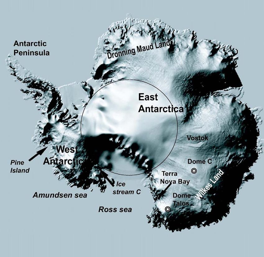
partie ouest du continent (Fig. 1) est d’un volume dix travers l’atmosphère ou la ionosphère...) il faut rajou-
fois moindre que la partie est, mais repose sur un socle ter des erreurs spécifiques, à savoir l’erreur causée par
très enfoncé sous le niveau de la mer, dont le flux géo- la pente de la surface qui décale le point d’impact et
thermique est beaucoup plus fort que pour la partie est celle causée par la pénétration de l’onde radar dans la
[26,45]. Certains auteurs soupçonnent que l’Antarctique neige [39]. La Fig. 4, qui montre la différence d’es-
de l’Ouest est potentiellement instable. Il a d’ailleurs timation de la topographie entre les deux fréquences
connu dans le passé des fluctuations de masse beaucoup différentes de l’altimètre d’Envisat, illustre la pénétra-
plus forte que la partie est. tion de l’onde dans la neige. L’analyse de six années de
Estimer le bilan de masse peut consister à comparer données ERS [57] suggère aussi une relative stabilité de
la quantité de neige qui tombe et la quantité de glace la partie ouest (−1 ± 53 km3 an−1 ) et un bilan négatif
rejetée dans l’océan (voir Section 2). On peut aussi di- pour la partie est (−59 ± 60 km3 an−1 ). Cependant, la
rectement estimer l’effet intégré sur la topographie, soit comparaison, purement relative, avec des données plus
en mesurant les variations de volume par altimétrie, soit anciennes de Seasat (1978) montre que la partie ouest
en comparant les taux d’accumulation de neige avec les se déforme légèrement, certaines zones en amont des
vitesses d’enfouissement (voir Section 3). On peut aussi grands fleuves émissaires semblant encore subir l’effet
modéliser les précipitations neigeuses et l’écoulement de la hausse des océans ayant eu lieu au début de l’Ho-
de la glace, afin de prédire l’évolution future (voir Sec- locène [34].
tion 4). La pause de coffee can ou de « boîte à café » à plu-
De nombreuses raisons rendent ce travail délicat : le sieurs dizaines de mètres de profondeur, dont on mesure
continent est grand et difficile d’accès, les mesures in la vitesse d’enfouissement, permet de mesurer directe-
situ y sont rares, les mesures satellites sont peu validées ment l’équilibre de la surface par comparaison avec les
et peu étalonnées. Les processus physiques, climato-
taux d’accumulation locaux. Plusieurs de ces « boîtes à
logiques et dynamiques sont complexes et encore peu
café » ont été installées entre dôme C, dôme Talos et
connus. Les conditions limites ne sont pas suffisamment
Terra Nova Bay (voir Fig. 1). Dans le secteur étudié, la
connues. La variabilité spatio-temporelle est extrême-
surface semble être en équilibre, mais l’incertitude est
ment forte. Enfin, les temps de réaction face à une per-
très forte, la forte variabilité spatiale des taux d’accu-
turbation climatique sont très variés (voir Fig. 2), très
mulation de neige étant le problème majeur qui se pose
faibles en ce qui concerne les précipitations, extrême-
pour l’interprétation de ces observations.
ment longs en ce qui concerne l’écoulement de la glace.
Ainsi, l’Antarctique n’est toujours pas stabilisé depuis
Modélisation
le réchauffement climatique du début de l’Holocène.
Analyse des flux La difficulté majeure pour la modélisation des ca-
lottes polaires, en dehors de la complexité des méca-
Le flux de neige entrant est estimé sur la totalité nismes atmosphériques et dynamiques et de la mau-
d’un bassin et les flux de glace sortant sont estimés vaise connaissance de la majorité des paramètres, ré-1086 F. Rémy, M. Frezzotti / C. R. Geoscience 338 (2006) 1084–1097
side dans la diversité des temps de réaction (Fig. 2). Il ment de l’atmosphère polaire austral, mais ceci n’est en
faut, en effet, non seulement connaître les valeurs des aucun cas observé à l’heure actuelle.
forçages actuels, mais aussi des forçages passés, taux
d’accumulation de neige, limites côtières, température... 1. Introduction
Un état donné simulé n’est représentatif et stationnaire
qu’après une modélisation de plusieurs centaines de The mass balance of the Antarctic ice sheet is one
milliers d’années [44]. Il est d’usage de discerner le si- of the sources of uncertainty about the sea-level rise
gnal lié aux altérations climatiques actuelles (positif ?) and it is possible that this will be even truer in the fu-
du signal résiduel dynamique lié au réchauffement du ture [29,55]. Moreover, calculations with global climate
début de l’Holocène (négatif ?). Les incertitudes pour le models (GCMs) indicate that warming in the polar areas
signal actuel viennent essentiellement de la discordance will be enhanced by a factor of 2 or 3. One of the con-
entre les modèles prévoyant un réchauffement austral et sequences of such an increase in polar warming could
les données suggérant un refroidissement. Celles pour be a sea-level rise due to melting of the Greenland and
le signal résiduel viennent, pour une bonne part, de la Antarctic ice sheets.
manière de prendre en compte, dans les modèles, l’effet This paper focuses on the mass balance of the
des grandes plates-formes de glace qui bordent le conti- Antarctic ice sheet (Fig. 1). With a surface area of
nent. Le consensus actuel veut que l’on assiste encore 14 million km2 and an average ice thickness of 2200 m,
quelque temps à une très légère diminution du volume it accounts for 90% of the terrestrial ice, which would
de glace consécutive aux effets résiduels, avant que raise the sea level by 70 m if it melted. Each year, about
l’augmentation des taux d’accumulation causée par un 2200 gigatonnes of snow fall on the Antarctic ice sheet
réchauffement potentiel de la région australe ne vienne and sink toward deeper layers, where it slowly changes
inverser la tendance [21]. Les discordances entre mo- into ice. The ice then flows toward the coast, where the
dèles et scénarios climatiques adoptés n’affectent essen- same quantity of ice is rejected to the ocean much later
tiellement que le moment où la tendance s’inverse. (Fig. 2). This annual balance corresponds to 6.5 mm of
Enfin, l’Antarctique est tellement inerte qu’il ne ré- sea level, so that a slight imbalance may have an impact
pond que lentement à des fluctuations climatiques ra- on sea-level change.
pides. L’effet cumulatif sur la calotte de la variabilité The behaviour of the West Antarctic ice sheet
des taux d’accumulation de neige peut être comparé à (WAIS), which would lead to a sea-level rise of 6 m
une marche au hasard, c’est-à-dire à l’addition de pe- if it melted, is more critical than that of the eastern part
tites perturbations aléatoires intégrées [31,34], où l’on because its bedrock is largely below the sea level and
peut s’éloigner fortement de la position initiale, sans rai- because, as demonstrated in recent works, its geother-
son physique déterministe. On montre qu’une variabilité mal flux is high, inducing warmer basal temperature
annuelle de 25% de la valeur moyenne a une chance than in the eastern part [26,45]. This western part is
sur cinq de générer un signal supérieur à 10% des taux thus suspected to be unstable and likely to suffer a large
d’accumulation sur plusieurs décennies (Fig. 5), ce qui
collapse, especially during warm periods. Finally, geo-
correspond à une évolution du niveau de la mer de
logical data indicate that the WAIS extended far away
0,65 mm an−1 .
from its current position during the last interglacial pe-
riod, unlike the eastern part, which appears to be very
Synthèse et conclusion
stable.
The mass balance problem can be easily understood
En dépit des incertitudes fortes, les deux moyens
with a simplified mass conservation equation:
d’observations du bilan de masse de l’Antarctique
(comparaison des flux entrants et sortants ou mesure dH /dt = −d(U H )/dx + b (1)
intégrée des effets sur la surface) montrent une relative
stabilité de la partie est et une légère diminution de la in which t is the time; the x axis is oriented from the
partie ouest, correspondant à une élévation du niveau de dome to the coast, in the ice-flow direction. U is the ver-
la mer de 0,15 à 0,20 mm an−1 . Cette perte de masse tically integrated ice-sheet velocity, H the ice thickness
est partiellement due au retrait des lignes d’ancrage de and b the mean local accumulation rate of snow.
la glace dans la zone de Pine Island (Fig. 1), causée par This equation states that imbalance between input
un réchauffement local. Cette perte pourrait être théo- mass (input ice flow and accumulation) and output (out-
riquement compensée par une augmentation des taux put flow) is counterbalanced by the change in height.
d’accumulation de neige, entraînée par un réchauffe- The actual mass balance can thus be estimated either byF. Rémy, M. Frezzotti / C. R. Geoscience 338 (2006) 1084–1097 1087 Fig. 1. Topography of the Antarctic ice sheet derived from the ERS-1 geodetic mission [38]. The circle shows the ERS inclination and the main locations mentioned in the text are shown. Fig. 1. Topographie de la calotte Antarctique déduite de la mission géodésique d’ERS 1 [38]. L’inclinaison d’ERS ainsi que les principaux lieux mentionnés dans le texte sont indiqués. measuring the difference between output and input (the – this huge continent is the coldest, highest, driest and component method, see Section 2) or by surveying the windiest continent on Earth. In situ measurements ice volume (left hand of Eq. (1), the integrated method, are still very sparse, and satellite remote sensing see Section 3). Temporal changes of the input and out- techniques are affected by the lack of validation, the put mass can also be modelled in order to predict future penetration of the radar wave within the snowpack changes (see Section 4). and the high variability of the surface roughness so Both snow accumulation and ice flow processes are that a lot of geophysical parameters are still dif- strongly temperature dependent, but with different time ficult to evaluate. For instance, as will be seen in lags. Warming of air temperature is supposed to rapidly Section 2.1, one of the most pertinent climate para- increase snow precipitation. On the contrary, changes in meters, the accumulation rate, has a very large un- air temperature slowly modify the ice temperature and certainty, leading to an equivalent error in the global hence also the rate of deformation when the temperature sea-level change of more than ±0.6 mm yr−1 %; change reaches a depth at which significant deformation – the physical processes are complex and not well occurs. This last process takes a very long time, more known. Physical processes linking climate and than several thousand years. (See Fig. 2 for the different snow precipitation are still being investigated. The time scales on which ice sheet mechanisms work.) parameters of the rheological law linking ice veloc- It is very difficult to estimate mass balance for the ity to the basal shear stress, surface slope and ice Antarctica ice sheet, for many reasons: temperature get a very large set of values [1,19],
1088                                     F. Rémy, M. Frezzotti / C. R. Geoscience 338 (2006) 1084–1097

Fig. 2. Ice-sheet mechanism and time-scale outline adapted from [33]. Surface melting, snow precipitation, sublimation, wind-driven sublimation,
and basal melting or refreezing are assumed to instantaneously react to climate change. Ice streams, outlet glaciers and ice-shelf dynamics are
assumed to react slowly to climate change, meaning between 100 and 1000 yr. On the contrary, ice flow, basal temperature and fusion isostasy take
a very long time to react, meaning that the time lag is between 10 000 to 100 000 yr.
Fig. 2. Les principaux mécanismes agissant sur la géométrie de l’Antarctique et les différents temps de réaction associés, adapté de [33]. La fonte
à la surface, les précipitations de neige, la sublimation ou les phénomènes de fonte–regel sous les plates-formes de glace réagissent pratiquement
instantanément à une variation climatique. En revanche, les fleuves de glace, les glaciers émissaires ou la dynamique des plates-formes réagissent
un peu plus lentement, environ 100 ou 1000 ans après la perturbation. Quant à l’écoulement de la glace, la température à la base de la calotte ou
l’isostasie, le temps de réaction est fort long, de l’ordre de 10 à 100 000 ans.

    which means that there is great discrepancy in ve-                         – as for any component of the global climate, the
    locity estimations. Also, much of the ice is trans-                          Antarctic climate has large space and time variabil-
    ported from the interior to the coast via fast-flowing                       ity. For instance, the annual precipitation variabil-
    ice streams. These streams dynamics are strongly                             ity is estimated at about 25% of the mean value.
    controlled not only by poorly-known bed condi-                               The large relaxation time of the ice sheet induces a
    tions, but also by basal temperature, water content,                         low-frequency response in this random fluctuation
    tills, etc.;                                                                 [30,40];
  – the boundary conditions are not fully known. Most                          – finally, the snow densification process is also a lim-
    of the ice is evacuated through floating ice shelves,                        itation. The relation between ice volume change,
    which means that the transition from grounded to                             as monitored by altimetry or topography surveys,
    floating ice, the grounding line, which determines                           and ice mass change which is directly related to
    the exact boundary of the ice sheet, is frequently not                       sea-level change and monitored by gravity mis-
    well located. Furthermore, the bedrock topography                            sion, requires knowledge of the snow density pro-
    and ice thickness that are two of the relevant para-                         file [37].
    meters for modelling ice dynamics are not known
    over huge sectors of a few tens of thousands of                              No claim is made here to an exhaustive review of
    square kilometres [27];                                                  Antarctica mass balance studies, but an attempt has been
  – due to the large thermal inertia of ice, the present                     made to consider different tools and results. The article
    state of the ice sheet is a result of its past history                   is thus structured around a discussion of these different
    over several climatic cycles. Consequently knowl-                        tools, namely: (1) the comparison between mass input
    edge of past climate forcing is an important con-                        and mass output, or the ‘component survey’, (2) the
    straint;                                                                 integrated measurement of the volume either through
F. Rémy, M. Frezzotti / C. R. Geoscience 338 (2006) 1084–1097 1089
satellite remote sensing or from in situ measurements,
(3) the ice sheet dynamics and heuristic or stochastic
modelling based on climate forcing.
2. The component survey
The component (or flux) approach to mass balance
consists of algebraically summing mass input, i.e. net
mass balance at the surface and the mass output of solid
ice from the ice sheet.
2.1. Input measurements
Snow accumulation or surface mass balance on the
Antarctic Plateau is the sum of precipitation, sublima-
tion/deposition and wind-blown snow. Its estimation by
compilation and interpolation work [16,54] has indi-
cated that surface mass balance estimates tend to con-
verge towards a common value, suggesting a residual Fig. 3. Subscene of Landsat ETM in false colour showing a plateau
error of less than 10% for the Antarctic ice sheet (equiv- area with megadunes. The arrow shows the prevailing wind direction.
alent to a sea-level rise of ∼0.6 mm a−1 ). However, These unexpected structures were recently discovered in a satellite
image. They are due to a feedback system between the cryosphere
ITASE research has indicated a high variability of sur- and the atmosphere [6,9].
face mass balance and also that single core, stake or
Fig. 3. Scène du satellite Landsat en fausse couleur montrant un
snow pit measurements are not representative of geo- champ de « mégadunes » sur le plateau Antarctique. La flèche indique
graphical/environmental characteristics of the site. The la direction prédominante du vent. Ces structures inattendues ont été
new data collected in the ITASE framework or associ- découvertes récemment, grâce à des observations par satellite. Elles
ated with projects for deep drilling surveys (Dome C, sont dues à une interaction entre la cryosphère et la neige [6,9].
DML, Siple Dome, US West Antarctica, Law Dome,
Dome Fuji, etc.) show systematic biases with respect to to the redistribution process (erosion/deposition) lead-
previous compilations of up to 65% [8,28]. Most of the ing to dune/sastrugi formation, but detailed field surveys
data for East Antarctica used for the snow surface com- have pointed out that the redistribution process is a local
pilation [16,54] were collected during the 1960s, using effect that has a strong impact on the annual scale vari-
snow pit stratigraphy, which generally overestimates ac- ability of accumulation (i.e. noise). The high variability
cumulation rates [31]. In addition, there are large gaps in of surface mass balance is due to ablation processes
data coverage, due to the very sparse distribution of in driven by katabatic winds (wind scouring, surface and
situ measurements (1860 accumulation data points for blowing sublimation); only megadunes and some occa-
about 12 million square kilometres, i.e. one data point sional transversal dunes show depositional features [8].
every 6500 km2 ), particularly in East Antarctica. The re-analysis of ECMWF (ERA) surface mass bal-
Moreover, satellite image analysis enables the dis- ance for the interior of the continent also yields signifi-
covery of unexpected surface features as shown in Fig. 3 cantly lower values than that provided by surface mass
(megadune, wide glazed surface, etc.) due to a feedback balance compilation [49]. Systematic negative ‘biases’
system between the cryosphere and the atmosphere between Atmospheric General Circulation Models and
[6,9]. Field observations have shown that the interac- surface mass balance compilations have been observed
tion of surface wind with subtle variations of surface in regions devoid of field observations or characterised
slope along the wind direction has a considerable im- by strong winds [15].
pact on the spatial distribution of snow on short and
long spatial scales [10]. Wind-driven ablation greatly 2.2. Output measurements
affects the surface mass balance. Our idea of a flat
ice sheet surface and homogeneous snow accumulation Remote sensing surveys by satellite and/or airborne
variability over the Antarctic ice sheet has radically al- are ideal tools [13,41] for evaluating the ice discharge.
tered. Most snow variability has previously been linked This is done by measuring ice thickness at the ground-1090 F. Rémy, M. Frezzotti / C. R. Geoscience 338 (2006) 1084–1097
ing line (with airborne Radio-Echo sounding, or free- Accurate knowledge of the surface mass balance is
board of floating ice from satellite altimetry) and by thus the most significant gap in current estimates of
measuring ice velocities (with InSAR or/and track- mass balance.
ing methods). These observations of the Antarctic Ice
Sheet in the last decade have identified recent unex- 3. Volume survey
pected changes, which are much more dynamic than had
previously been thought. Some glaciers are found to ac- A volume or elevation change survey (i.e. to deter-
celerate strongly, for instance the Pine Island Glacier mine values for the left term of Eq. (1)) is a direct way of
on the West Antarctic ice sheet is accelerating by estimating mass balance. This can be either done on the
45 m yr−1 [43], while others have been found to de- global scale with satellite altimetry or locally with sub-
celerate or even stop. mergence velocity estimation. Both methods are great
Rignot and Thomas [43] reviewed the mass budget tools for surveying elevation change, but the first one re-
of 33 Antarctic glaciers, using remote sensing measure- quires ground-based measurements to check the satellite
ments to determine the ice discharge at the grounding data and study the process involved in elevation change,
line with the most recent snow accumulation compi- while the second one only provides a local measurement
lations [16,54]. The authors pointed out that the West where markers have been installed.
Antarctic Ice Sheet is thinning in the west with a loss
of 72 km3 yr in the Admundsen Sea sector and that it is 3.1. Satellite altimetry
thickening in the north with a slight gain of 33 km3 yr−1
in the Ross Sea sector. The main reason for the posi- Since the launch of ERS-1 in 1992, the Antarctica ice
tive balance of this region is the stoppage of ice stream sheet can be surveyed with a radar altimeter to the north
C about 150 years ago and the continued slowing- of 81.5◦ S, which is the satellite inclination. However, a
down of the Whillians ice stream [43]. Nevertheless, lot of corrections have to be applied to take into account
the West Antarctic ice sheet is probably thinning on the tracker lag, the orbit restitution, the atmospheric de-
the whole (−48 ± 14 km3 yr−1 ). On the contrary, the lay, the slope-induced error or the solid tide (see for
mass imbalance of the East Antarctic Ice Sheet, esti- instance [35]). Moreover, due to the penetration of the
mated with 20 surveyed glaciers, is likely to be small waveform within the snow pack, temporal changes in
(+22 ± 23 km3 yr−1 ), and even its sign cannot be deter- surface scattering strongly affect the radar height mea-
mined yet. surements [24]. This error is very critical because the
snow pack and the surface characteristics may change
2.3. Limitation of the method from the meteorological scale to the long-term scale.
However, the surface topography of Antarctica, one of
Mass balance results are subject to large uncertain- the most relevant parameters for investigating ice sheet
ties both on the distribution of accumulation rate over dynamics and mass balance, can be mapped with an ac-
the basin and on the basin delimitation itself. Indeed, curacy of less than a metre in the central part of the
recent results [7,8,50] have pointed out that the ice di- continent, north of 82◦ S [39].
vide has migrated or has been encroached upon by other The ERS data were used to survey Antarctica from
basin systems, also on a relatively short timescale of a 1992 to 1996 [57]. The 5-year rate of elevation change
few hundred years. The current coastal ice flux does was mapped with a resolution of 1◦ × 1◦ . In order to
thus not correspond to the basin delimitation, as esti- decrease the noise, estimated to be 4 cm yr−1 over a
mated with the current topography. Fricker et al. [14] cell, the data were averaged over a correlation length
also pointed out that mass balance results are subject to of 200 km. The imbalance of West Antarctica was
large uncertainties in the distribution of accumulation found to be −59 ± 60 km3 yr−1 , whereas the imbalance
over the basin, such that current estimates of Antarc- of the East part was found to be −1 ± 53 km3 yr−1 .
tic accumulation rates are unsuitable for this type of A more recent study with 11 years of ERS data sug-
study; this is the most significant gap in current mass gests now a positive imbalance for the eastern part of
balance estimates. New data have shown that there is 45 km3 yr−1 [5]. This signal is correlated with an in-
currently no proven method of interpolating across the crease of precipitation and corresponds to of decrease
huge gaps remaining between existing snow accumula- of 0.12 mm yr−1 of the sea level. Nevertheless, neither
tion data. Acquisitions of more and more accurate field changes in snowpack characteristics nor snow densifi-
determinations of the Antarctic surface mass balance cation are taken into account in this study, so that this
are crucial. estimation is an upper limit of the mass change.F. Rémy, M. Frezzotti / C. R. Geoscience 338 (2006) 1084–1097 1091 An attempt was made to compare the observations using repeated geodetic surveys (GPS–DORIS), to de- of the Seasat altimeter, obtained in 1978 with those of termine the local rate of ice elevation change [17,20]. ERS-1, launched in 1992 over the common survey area The submergence velocity system is based on GPS sur- in the Wilkes Land north of 72◦ S, in order to take ad- veys of markers anchored some tens of metres deep vantage of the long time between the two missions [34]. in the firn. The markers have been frozen to the bore- Unfortunately no cross-calibration has ever been per- hole base using water and are connected to the surface formed between the two altimeters, so that only the rel- by steel cables that cannot stretch. These vertical ve- ative difference between the two topographical surveys locity measurements are then compared with the rate can be determined. The geographical changes in height of snow accumulation, determined from the different during the 14 years separating the missions have been sources (stake farm, fin core or snow radar profiling). mapped via an inverse technique that allows us to take Submergence velocity systems were installed during the whole altimetric error budget into account. Also the a transect Terra Nova Bay–Dome C (seven sites) and error due to changes in snow characteristics over time in Wilkes Land (D66-Talos Dome, eight sites) in 1998– was corrected for after the inversion. In a belt between 1999 and during the 2001–02 ITASE traverse. A first 70◦ S and 72◦ S and between 150◦ E and 80◦ E, a preci- repetition of these measurements along the Terra Nova sion of better than 40 cm, e.g. 2.8 cm yr−1 for the trend Bay-Dome C transect was performed and elaborated us- was found for the surface elevation change. The mapped ing the GIPSY-OASIS II software [56]. In this study, change in height between the two missions suggests a the horizontal position accuracy is about ±7 cm, and rise of the western part of the sector (150 E–140 E) and the vertical accuracy is around ±11 cm (with uncertain- of the high-altitude region, corresponding respectively ties at 95% confidence level). In an analysis by Vittuari to a positive imbalance of 20% and 25%. et al [56], Tambora’s marker (1816) was used based on The major altimetry error is probably due to the sur- nssSO4 core stratigraphy. Different authors [17,18,20] face slope. This error is not reproducible from one track have pointed out that errors in submergence ice veloc- to the other because the across-track orbit fluctuations ity measurements are dominated by temporal variability induce large noise. This error strongly increases with in snow accumulation rates. On the contrary, Frezzotti the surface slope, which means that it is not possible to et al. [12] pointed out that the spatial variability of snow survey the coastal areas that are probably more sensi- accumulation at the kilometre scale, derived from snow- tive to climate change. The second error, dominant in radar and cores, is one order of magnitude higher than the central part, is due to the variation of the snowpack its temporal variability (20–30%) at the century scale. characteristics over all temporal time scales. The recent At the submerged pole sites, snow accumulation rates launch of the Envisat satellite now makes it possible, for derived with different time periods (four years, stake the first time ever, to survey the ice caps with a dual- farm; 40 years, tritium marker level; 180 years, Tamb- frequency altimeter in order to better understand the ora marker) differ significantly due to the horizontal ice penetration error. The difference in height as seen by the displacement and to the high spatial variability of snow two altimeters working with different radar frequencies accumulation correlated with a wind-driven sublimation could be as much as 2 m (see Fig. 4 and [25]) suggest- process. ing a relation between penetration and frequency. The The calculated rates of thickness change were all survey of change in this difference may allow detect- quite small and the formal uncertainties were close to ing modification in penetration. Finally, snow densifi- the estimated thickness changes. Analysis of submer- cation may have created a bias between mass change gence velocity using different methods and time scales (what we need) and volume change (what we are look- yielded different results. The sites with high snow accu- ing for with altimetry). Densification rate may change mulation variability (>10%) showed thinning, whereas with environmental conditions so that another error may the sites with accumulation variability
1092                                     F. Rémy, M. Frezzotti / C. R. Geoscience 338 (2006) 1084–1097

Fig. 4. Difference of altimetric height as seen by both antenna of the dual-frequency altimeter of Envisat (one in Ku band at 13.6 GHz, the other in
S band at 3.6 GHz) [25]. The difference is due to the difference between penetrations of both radar waves within the dry and cold snowpack. This
gives an idea of how large the penetration error could be. Since the penetration error is due to the snowpack characteristics, it could change with
time and induce an erroneous signal on an altimetry trend. This error is probably the dominant one in the interior of the Antarctic.
Fig. 4. Différence d’appréhension de la topographie, vue par les deux fréquences de l’altimètre d’Envisat (l’une en bande ku ou 13,6 GHz, l’autre
en bande S à 3,6 GHz) [25]. La différence est due à la différence de pénétration des ondes radar dans les deux fréquences. La figure illustre
l’importance de cette erreur. Par ailleurs, l’erreur due à la pénétration n’est pas reproductible, puisqu’elle dépend des conditions du manteau
neigeux (température, taille de grains de neige...) ; elle peut donc entraîner un biais sur l’estimation des tendances altimétriques.

sider aeolian processes when selecting optimum sites                         seems to indicate steady-state conditions in this part
for the submergence velocity system, because slope                           of East Antarctica, but due to the very slow submer-
variations of even a few metres per kilometre have a                         gence velocity (a few cm yr−1 ) and the low accumula-
significant impact on winds and on the snow accumu-                          tion rate (from 100 to 30 kg m2 yr−1 ), the uncertainty is
lation process. As a consequence, a lack of information                      high.
on local conditions can lead to an erroneous defini-
                                                                             4. Ice sheet modelling
tion of climatic conditions based on the interpretation
of snow accumulation and submergence velocity alone.
                                                                                Few authors have attempted to model mass balance
According to our observations, the sites with high stan-                     of the ice sheet according to different climate warming
dard deviation of spatial variability in snow accumula-                      scenarios, in order to predict their future. A review of
tion are not useful sources of information on temporal                       such models can be found in [53]. The model of Huy-
variations in snow accumulation and also submergence                         brechts and de Wolde [21] is one of the most recent
velocity, because it is very difficult or impossible to                      and complete ones. Their dynamic and ablation models
interpret the data when the snow originated under differ-                    were used by the Intergovernmental Panel on Climate
ent snow accumulation conditions. However, the result                        Change (IPCC) to derive the sea-level projections de-
F. Rémy, M. Frezzotti / C. R. Geoscience 338 (2006) 1084–1097 1093
scribed in the third assessment report [3]. These models between −0.5 to −1.5 mm yr−1 . However, in the high
generate ice sheet geometry for a given set of changes scenario case, due to a high melting rate in the marginal
in sea level, surface temperature and net surface balance zone and warm ice shelves, the trend would be reversed
(precipitation minus ablation). in 500 years.
The last IPCC report used the Huybrechts and de
4.1. Modelling the net surface mass balance Wolde model to project the evolution of sea level with
another climatic scenario. This new estimation gave a
As already mentioned, short-term mass balance greater increase in precipitation.
changes are due to the net surface mass balance. Un- However these results are questionable. First, an in-
til now, the usual assumption has been that precipitation crease in snow precipitation coupled with an increase
changes are related to the actual precipitation amount in temperature and/or wind could increase the sur-
weighted by change in temperature, according to the face mass balance in the inner part of East Antarctica
saturation vapour pressure law of Clausius–Clapeyron. alone, while inducing a decrease in surface mass bal-
The difficulty and the uncertainty inherent in this ance in the windy areas that account for 90% of the
method are due to the estimation of the current tem- Antarctic surface [11]. Second, Van der Veen [53] has
perature change, of the current average accumulation shown that the observations on which these models are
rate and to the parameterization of the relation between based are not relevant enough and that the models do
temperature and precipitation changes. The relation is not capture all relevant physical processes. In partic-
derived from ice core data by comparing past temper- ular it is difficult to take into account changes in at-
ature variations with past accumulation variations [4]. mospheric circulation patterns, which play an important
Precipitation increase is thus estimated at between 4 and role. Third, an analysis of 20 years of microwave emis-
10% per degree of warming. sivity of the Antarctic surface has shown that the cu-
Note that the fraction of precipitation on the grounded mulative melting surface has decreased by 1.8% yr−1 ,
ice that is returned to the atmosphere through subli- with a confidence of 1% yr−1 , resulting from a mean
mation in Antarctica is not negligible [7] and that the (at least) summer cooling of the continent [48]. This re-
sublimation process is not explicitly included in numer- sult is in contradiction with the climate forcing scenario
ical weather prediction and general circulation models used.
[15]. Moreover, changes in precipitation can also be in-
duced by changes in atmospheric circulation as has been 4.2. Background trend: dynamic modelling
suspected by [23]. In any case, it is clear that the rela-
tion between precipitation and climate is not trivial and The processes controlling the shape of the Antarctic
probably depends on the considered time-scale, climatic ice sheet are the grounding line migration, the internal
period and ice sheet geometry. For all these reasons, the structure and the thermo-mechanical coupling between
uncertainties on the rate of precipitation increase due to velocity and temperature. The three components of the
climate warming could be very great [53]. ice sheet: the grounded ice, the ice streams and the ice
Ablation is deduced from the relation between posi- shelves, are taken into account. Due to the large iner-
tive degree days and melt rate or from an energy balance tia of ice, especially of ice internal temperature, mod-
model. However, there are never many positive degree elling of the current background evolution of the ice
days in Antarctic and these occur only near the coast sheet has to be initialized during several glacial cy-
[48]. Even for the middle warming scenario of Huy- cles. Inadequate knowledge of past conditions is one
brechts and de Wolde [21], the mean ablation in 200 of the major limiting factors on confidence in the ac-
years will be still less than 5% of the total loss. tual state, with others being the assumption about the
Finally, both precipitation and melting are parame- dynamical processes, rheological law or ice stream pa-
terized in terms of temperature which is derived from rameterization. Over these timescales, grounding line
a coupled climate and ocean model. For instance, the migration due to sea level change mostly controls ice
forcing used in the Huybrechts and de Wolde model [21] geometry, while snow accumulation controls ice vol-
yields a mean increase of the Antarctica surface temper- ume. Due to the long integration time and to the grid
ature of between 2 ◦ C (low scenario) to 8 ◦ C (high sce- size (40 km), the ice streams are not treated individu-
nario) within the next 150 years. Depending on different ally. Because slower flowing ice contributes slowly to
scenarios, the ice sheet thickening corresponds to a de- sea-level change, this grid coarsening induces models
crease in sea level over the next 200 years of between to respond more slowly than actual ice sheets [2]. The
10 and 30 cm, corresponding to a sea-level change of temperature is parameterized with the help of the sur-1094 F. Rémy, M. Frezzotti / C. R. Geoscience 338 (2006) 1084–1097
face height and the accumulation rate with the help 4.3. Stochastic modelling
of the temperature. Past accumulation is deduced as
previously explained. These models are usually tested Throughout this paper, we have seen how large and
from available geological and glaciological field data; problematic the snow-accumulation fluctuations are.
see [44]. Another induced effect is that the long relaxation time of
In Ritz’s model [44], the Vostok area is still increas- the ice sheet induces a low-frequency response to these
ing due to the enhanced accumulation rate, as the warm- random fluctuations of snow accumulation. Short-term
ing of the ice has not yet reversed the trend. In the changes in the volume of ice sheets as analyzed, for in-
Huybrechts and de Wolde model [21], the retreat of stance by radar altimetry or short-term change in the
the WAIS takes place between 9000 and 4000 years mass of the ice sheets as measured by gravity satellite
before the present day. For both models, the Antarc- may not be related to long-term climatic change. Since
tic ice sheet is still reacting to the Holocene warming, the time scale of the response is great in comparison to
which leads to an actual equivalent increase of sea level the average human lifetime, the effect of these random
of 0.4 mm yr−1 , mostly due to the retreat of the WAIS fluctuations on sea-level change may be important even
groundling line. For the next millennium, the predicted if they are not linked to climatic change [30,40,51].
sea level rise is 20 cm, corresponding to a mean rate of Indeed, the mass conservation equation can be re-
0.2 mm yr−1 . written as:
Note that at the century–millennium timescale, the dH /dt = H /Tr + b (2)
dynamic response of the ice shelves may also play
a role. Taking into account the ice shelves’ behav- in which stands for the anomaly of the parameters
iour mostly acts on the timescale where the growth of with respect to their mean values and Tr is the relax-
Antarctica, following a warming is reversed. A warmer ation time. Rémy et al. [40] developed an analytical
ice shelf will deform more rapidly, leading to upslope expression for the relaxation time, which is then found
thinning and acceleration. However, it is very difficult to depend on the ice thickness, surface slope and rhe-
ological parameters and to vary from a few thousands
to model ice shelf dynamics and the greatest limita-
years near the coast to a few hundred thousand years
tion is temperature parameterization. Another constraint
in the interior. They applied a stochastic perturbation
is basal melting above the ice shelf. New observations
of accumulation rate anomaly assuming 25% of vari-
have revealed that the basal melting rate experienced
ability with respect to the mean accumulation rate and
by large outlet glaciers near their grounding line is one
looked at the evolution of the change in height. They
order of magnitude greater than had previously been
found a 20% chance of generating an artificial absolute
assumed [13,41]. The ice shelf melting rate is posi-
mass trend greater than 10% of the accumulation rate
tively correlated with thermal forcing, increasing by (expressed in ice equivalent), i.e. generating a sea-level
1 m yr−1 for each 0.1 ◦ C rise in ocean temperature. rise of 0.65 mm yr−1 .
When deep water has direct access to the grounding Moreover, when the densification process linking
line, glaciers and ice shelves are vulnerable to ongoing volume and mass is taken into account, the induced
increases in ocean temperature. For instance, accelera- trend in elevation, as measured by satellite altimetry, is
tion of Admundsen Coast glaciers increased mass flux enhanced [37]. One now has a 30% chance of having
to ice shelves, while ice shelves have thinned. This sug- an artificial absolute trend greater than 20% of the accu-
gests that basal melting increases probably due to a mulation rate. The scatter of the induced trends is such
penetration of the warm Circumpolar Deep Water [2]. that the sign of the ice mass trend may be opposite to the
Ocean temperature directly seaward of Antarctic’s con- sign of the measured volume trend (see Fig. 5). The im-
tinental shelf break has risen by ∼0.2 ◦ C over recent pact of this climatic noise increases when the frequency
decades, which is sufficient to increase basal melting by of the variability decreases.
∼2 m yr−1 [42]. The conclusion is that we need to know the ‘recent-
Finally, it should be noted that some authors argue past’ variability in order to eliminate the residual error
that grounding line instability has been an important due to snow densification and accumulation rate fluctu-
factor in the collapse of palaeo-ice sheets and may play ations, above all in areas of high densification, namely
such a role in the future [17]. Titus and Narayanan [47] in the coastal areas. At least 10 years of data are needed
estimated at 5% the chance of this instability, making a to reduce the induced error by a factor of 6. Longer se-
substantial contribution to sea level of up to 16 cm in ries do not significantly reduce the error for the surface
the next century. trend estimation.F. Rémy, M. Frezzotti / C. R. Geoscience 338 (2006) 1084–1097 1095
the component survey method indicates a slight posi-
tive imbalance of 22 ± 23 km3 yr−1 (−0.065 mm yr−1
eq. s.l.), while survey by altimetry gives an upper limit
of twice this value and the coffee-can technique indi-
cates steady-state conditions in the surveyed sector of
East Antarctica. The model finds a slight negative im-
balance for this part due to the actual response of the
warming of the Holocene, as the signature of this sig-
nal was indeed observed with altimetry analysis. For
the western part, the component survey suggests a neg-
ative imbalance of 48 ± 14 km3 yr−1 (+0.14 mm yr−1
eq. s.l.) and the altimetry survey a negative imbalance of
Fig. 5. Fluctuations of ice mass (in bold) and of ice elevation (shown
by dotted line) due to short-scale random fluctuations of 25% of the 59 ± 60 km3 yr−1 (+0.18 mm yr−1 eq. s.l.), which may
mean accumulation rate (i.e., 16.6 cm yr−1 ). The process is initialised be explained by the retreat of ice shelves. These obser-
for 1000 years before the time t = 0 of the plot. Note that in one place vations, namely a slight increase of the east part and a
a 1-m increase of the topography can occur over 30 yr, without any significant decrease of the western part, have been re-
climatic significance.
cently confirmed by the analysis of 2.5 yr of Grace [32].
Fig. 5. Fluctuations locales en terme de masse (en gras, autrement Modelling of the Antarctica ice sheet [21] suggests
dit avec une densification instantanée) et d’altitude (en pointillé, au-
trement dit avec un taux de densification moyen), causées par des
that the current response of the Antarctica ice sheet
fluctuations aléatoires de 25% du taux d’accumulation moyen en An- is dominated by the background trend due to the re-
tarctique (c’est-a-dire 16,6 cm an−1 ). Le processus stochastique a été treat of the grounding line, leading to a sea-level rise
initialisé durant 1000 ans avant l’expérience. Remarquer que l’on peut of 0.4 mm yr−1 over the short-time scale (100 yr). This
observer une élévation moyenne de 1 m en 30 ans par ce processus, component is again found to be dominant during the
sans aucun lien avec les conditions climatiques.
following centuries, depending on the climate scenario.
Later, the precipitation increase will counterbalance this
Note that this combined effect of fluctuations in residual signal, leading to a thickening of the ice sheet
snow densification and random snow accumulation rate and thus a decrease in sea level. Taking into account
only affects the interpretation of surface elevation trend. the low and middle scenarios leads to a decrease in sea
Measurements taken using the coffee-can technique are level over the next millennium, while the high scenario
not affected by the snow densification process. inverses the trend in 500 years due to the grounding-line
Other random fluctuations, such as outlet boundary retreat. It should be noted that the time when the trend
conditions can also affect the shape of the Antarctic ice is reversed not only depends on the climatic scenario,
sheet [36,52]. Indeed, these outlet flow boundary pertur- but also on the ice shelves modelling, basal melting rate
bations are transmitted toward the inland ice sheet. The beneath ice shelves being the most critical factor to be
induced inland undulation wavelength and transmission estimated.
increase with the temporal wavelength of the perturba- However, these determinist models do not take into
tion, so that short time scale perturbations are strongly account the stochastic fluctuations of the forcing given
filtered [36]. However, because outlet perturbations are the inertia of the ice sheet. For instance, taking random
poorly quantified, it is difficult to predict their impact fluctuations of snow accumulation rate into account
on sea-level change. However, an analysis of anomalies alone yields a probability of a present-day induced sea
in ice sheet topography suggests that in some places, level rise of between 0.5 and 1 mm yr−1 over a 30-year
the actual response to a past outlet perturbation can be time scale at 10% ± 10% [40].
suspected, which means that the interpretation of local Both observations and modelling are still not reliable
elevation change may be erroneous [36]. enough. Let us point out some limitations and problems
that should be carefully considered.
5. Synthesis and conclusion The more critical factor is probably the surface mass
balance, which varies from location to location due to
Observations of the Antarctica ice sheet suggest that interaction between precipitation and wind driven by
the East Antarctica ice sheet is nowadays more or less slope along wind direction [9,11]. One of the major un-
in balance, while the West Antarctica ice sheet exhibits expected discoveries regarding cryosphere/atmosphere
some changes likely to be related to climate change and interaction was indeed made in the remotest part of
is in negative balance. For the East Antarctica ice sheet, the East Antarctic Ice Sheet with the discovery of the1096 F. Rémy, M. Frezzotti / C. R. Geoscience 338 (2006) 1084–1097
megadunes [6,9]. Major gaps in our knowledge of the level, in: J.T. Houghton, Y. Ding, D.J. Griggs, M. Noguer, P. van
temporal and spatial variability processes and of the ex- der Linden, X. Dai, K. Maskell, C.I. Johnson (Eds.), Climate
Change 2001: The Scientific Basis. Contribution of Working
act relation between climate change and precipitation
Group I to the Third Assessment Report of the Intergovernmental
change prevent us from producing a reliable estimate of Panel on Climate Change, Cambridge University Press, Cam-
current surface mass balance and from predicting its fu- bridge, UK, 2001, pp. 639–693.
ture trend. [4] D. Dalh-Jensen, S.J. Johnsen, C.U. Hammer, H.B. Clausen,
From the point of view of ice sheet dynamics, obser- J. Jouzel, Past accumulation rates derived from observed annual
vations of the Antarctic Ice Sheet over the last decade layers in the GRIP ice core from Summit, Central Greenland,
in: W.R. Peltier (Ed.), Ice in the Climate System, in: NATO
have identified recent unexpected changes, which are ASI Series I, vol. 12, Springer-Verlag, Berlin, Heidelberg, 1993,
much more dynamic than previously thought. Thus our pp. 517–532.
idea of a slowly evolving Antarctic ice sheet is radically [5] C.H. Davis, Y. Li, J.R. McConnell, M.M. Frey, E. Hanna,
changing [22]. However, the models lack some of the Snowfall-driven growth in East Antarctic Ice Sheet Mitigates re-
physical processes that may explain these unexpected cent sea-level rise, Science 308 (2005) 1898–1901.
changes. For instance, a limitation on predicting the fu- [6] M.A. Fahnestock, T.A. Scambos, C. Shuman, R.J. Arthern, D.P.
Winebrenner, R. Kwok, Snow megadune fields on the East
ture with respect to actual measurements and knowledge Antarctic Plateau: extreme atmosphere–ice interaction, Geophys.
lies in the effect of ice-shelf retreat on upslope glaciers. Res. Lett. 27 (20) (2000) 3719–3722.
It may be argued either that ice-shelf retreat has little [7] M. Frezzotti, G. Bitelli, P. de Michelis, A. Deponti, A. Fori-
effect on glaciers or that the breaking up of the ice- eri, S. Gandolfi, V. Maggi, F. Mancini, F. Rémy, I.E. Tabacco,
shelf will accelerate. Considerable improvements are S. Urbini, L. Vittuari, A. Zirizzotti, Geophysical survey at Talos
Dome (East Antarctica): The search for a new deep-drilling site,
also needed, in particular for characterizing fast mov-
Ann. Glaciol. 39 (1) (2004) 423–432.
ing outlet glaciers. The first results with ICEsat on the [8] M. Frezzotti, O. Flora, Ice dynamics and climatic surface para-
glaciers of the Ross embayment suggest that we can meters in East Antarctica from Terra Nova Bay to Talos Dome
hope a very good precision with a very fine space reso- and Dome C: ITASE Italian Traverses, Terra Antarctica 9 (1)
lution [46]. Lastly, due to numerical limitations, small- (2002) 47–54.
scale features such as fast glaciers are poorly taken [9] M. Frezzotti, S. Gandolfi, F. La Marca, S. Urbini, Snow dune and
glazed surface in Antarctica: new field and remote sensing data,
into account, so that ice sheet modelling underestimates
Ann. Glaciol. 34 (2002) 81–88.
rates of changes [2]. [10] M. Frezzotti, S. Gandolfi, S. Urbini, Snow megadune in
The ICEsat satellite, launched in 2003, will enable Antarctica: Sedimentary structure and genesis, J. Geophys.
measuring of ice sheet mass balance, but on a small Res. 107 (D18) (2002) 4344, doi:10.1029/2001JD000673.
temporal scale, which is insufficient for inferring long- [11] M. Frezzotti, M. Pourchet, O. Flora, S. Gandolfi, M. Gay,
term trends. Grace, launched in 2002, will give access S. Urbini, C. Vincent, S. Becagli, R. Gragnani, M. Propos-
ito, M. Severi, R. Traversi, R. Udisti, M. Fily, New estima-
to change in ice mass. By combining this data with the tions of precipitation and surface sublimation in East Antarctica
ERS and Envisat series, uncertainty with respect to ice from snow accumulation measurements, Clim. Dynam. (2004),
sheet mass balance will be reduced. doi:10.1007/s00382-004-0462-5.
In the future, the launch of several satellites dedi- [12] M. Frezzotti, M. Pourchet, O. Flora, S. Gandolfi, M. Gay,
cated to the study of the ice sheet may further our un- S. Urbini, C. Vincent, S. Becagli, R. Gragnani, M. Proposito,
M. Severi, R. Traversi, R. Udisti, M. Fily, Spatial and temporal
derstanding of the physical processes acting on ice sheet
variability of the surface mass balance in East Antarctica from
and of its actual state. Unhappily due to a launch failure, traverse data, J. Glaciol. (in press).
the Cryosat satellite, devoted for the survey of polar re- [13] M. Frezzotti, I. Tabacco, A. Zirizzotti, Ice discharge of eastern
gions, is postponed. Carisma mission, a P-band radar Dome C drainage area, Antarctica, determined from airborne
designed to sound the ice sheet, will provide us with ex- radar survey and satellite image analysis, J. Glaciol. 46 (153)
act ice thickness and volume, and will detect internal ice (2000) 253–273.
[14] H. Fricker, R. Warner, I. Allison, Mass balance of the Lam-
layering, which will be of great help for ice-sheet mod-
bert Glacier–Amery Ice shelf system, East Antarctica: a com-
elling. parison of computed balance fluxes and measured fluxes,
J. Glaciol. 46 (155) (2000) 561–570.
References [15] C. Genthon, G. Krinner, The Antarctic surface mass balance and
systematic biases in GCMs, J. Geophys. Res. 106 (2001) 20653–
[1] R.B. Alley, Flow-law hypotheses for ice-sheet modeling, 20664.
J. Glaciol. 38 (1992) 245–256. [16] M.B. Giovinetto, H.J. Zwally, Spatial distribution of net surface
[2] R.B. Alley, P.U. Clark, P. Huybrechts, I. Joungin, Ice sheet and accumulation on the Antarctic ice Sheet, Ann. Glaciol. 3 (2000)
sea-level changes, Science 310 (2005) 456–460. 171–178.
[3] J.A. Church, J.M. Gregory, P. Huybrechts, M. Kuhn, K. Lam- [17] G.S. Hamilton, I.M. Whillans, Local rates of ice-sheet thickness
beck, M.T. Nhuan, D. Qin, P.L. Woodworth, Changes in sea change in Greenland, Ann. Glaciol. 35 (2002) 79–83.Vous pouvez aussi lire