Démonstration expérimentale d'un avion autopiloté électrique contraint par un câble attaché au sol - Université de ...
←
→
Transcription du contenu de la page
Si votre navigateur ne rend pas la page correctement, lisez s'il vous plaît le contenu de la page ci-dessous
UNIVERSITÉ DE SHERBROOKE
                 Faculté de génie
          Département de génie mécanique

 Démonstration expérimentale d’un avion
autopiloté électrique contraint par un câble
               attaché au sol

               Mémoire de maitrise
            Spécialité : génie mécanique

                Bruno Chapdelaine

           Sherbrooke (Québec) Canada

                   Janvier 2021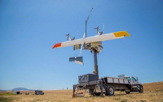
MEMBRES DU JURY

    David RANCOURT
         Directeur

 Alexis LUSSIER DESBIENS
         Évaluateur

   Jean de LAFONTAINE
         Évaluateur
RÉSUMÉ Les aéronefs à décollage et atterrissage vertical (VTOL) sont essentiels pour les services d’urgence, le transport de marchandise et la mobilité aérienne. Les récentes avancées en systèmes autonomes et en motorisation électrique ont ravivé le développement de ce type de véhicule. Les compagnies novatrices se concentrent principalement sur le développement de concepts de type multi-rotor qui souffrent d’une faible efficacité en vol stationnaire et en vol vers l’avant. Le nouveau concept d’un aéronef VTOL avec un rotor composé d’avions autonomes attachés par câble permettrait de lever des charges de façon plus efficace que les aéronefs VTOL actuels. Dans ce mémoire, un modèle de simulation dynamique et un banc d’essai expérimental d’un avion attaché par câble sont présentés. Le modèle dynamique permet de développer le système de contrôle de l’aéronef expérimental et de prédire les performances du système. Les essais expérimentaux démontrent que le système de contrôle est capable de stabiliser le véhicule à l’état désiré pour l’acquisition de données. Le véhicule est capable de lever une charge équivalente à 4 fois son poids à vide et d’atteindre un ratio de levage de 14 g/W en régime permanent. Le modèle dynamique prédit correctement la dynamique et les performances du système. Mots-clés : Véhicules aériens autonomes, Avion, Hélicoptère, Simulation dynamique, Contrôle embarqué
TABLE DES MATIÈRES

1 INTRODUCTION                                                                                                                 1
  1.1 Mise en contexte et problématique . . . . . . . . . . . . . . . . . . . . . . .                                          1
  1.2 Plan du document . . . . . . . . . . . . . . . . . . . . . . . . . . . . . . .                                           2

2 ÉTAT DE L’ART                                                                                                                3

3 QUESTION DE RECHERCHE                                                                                                        9
  3.1 Objectifs du projet de recherche . . . . . . . . . . . . . . . . . . . . . . . .                                         9
  3.2 Contributions originales . . . . . . . . . . . . . . . . . . . . . . . . . . . .                                        10

4 MODÈLE, VALIDATION ET RÉSULTATS                                                                                             11
  4.1 Introduction . . . . . . . . . . . . . . . . . .    .   .   .   .   .   .   .   .   .   .   .   .   .   .   .   .   .   13
  4.2 Experimental Setup . . . . . . . . . . . . . .      .   .   .   .   .   .   .   .   .   .   .   .   .   .   .   .   .   15
  4.3 Simulation Model . . . . . . . . . . . . . . .      .   .   .   .   .   .   .   .   .   .   .   .   .   .   .   .   .   17
      4.3.1 Dynamics Model . . . . . . . . . . .          .   .   .   .   .   .   .   .   .   .   .   .   .   .   .   .   .   17
      4.3.2 Aerodynamics Model . . . . . . . . .          .   .   .   .   .   .   .   .   .   .   .   .   .   .   .   .   .   20
      4.3.3 Controller Model . . . . . . . . . . .        .   .   .   .   .   .   .   .   .   .   .   .   .   .   .   .   .   21
  4.4 Results . . . . . . . . . . . . . . . . . . . . .   .   .   .   .   .   .   .   .   .   .   .   .   .   .   .   .   .   22
      4.4.1 Tests description . . . . . . . . . . .       .   .   .   .   .   .   .   .   .   .   .   .   .   .   .   .   .   22
      4.4.2 Controller performance . . . . . . . .        .   .   .   .   .   .   .   .   .   .   .   .   .   .   .   .   .   23
      4.4.3 Lifting capabilities . . . . . . . . . .      .   .   .   .   .   .   .   .   .   .   .   .   .   .   .   .   .   24
      4.4.4 Lifting efficiency . . . . . . . . . . .      .   .   .   .   .   .   .   .   .   .   .   .   .   .   .   .   .   26
  4.5 Conclusion . . . . . . . . . . . . . . . . . . .    .   .   .   .   .   .   .   .   .   .   .   .   .   .   .   .   .   28

5 CONCLUSION                                                                                                                  29

A DONNÉES D’EFFICACITÉ EN VOL STATIONNAIRE                                                                                    31

LISTE DES RÉFÉRENCES                                                                                                          33

                                            v
vi TABLE DES MATIÈRES
LISTE DES FIGURES

 1.1    Représentation schématique de deux configurations de rotor . . . . . . . .            2

 2.1    Représentation schématique de la méthode de transport de charge par deux
        avions brevetée par Wilson en 1981 . . . . . . . . . . . . . . . . . . . . . .       3
 2.2    Centrifugally Stiffened Rotor . . . . . . . . . . . . . . . . . . . . . . . . . .    4
 2.3    Alcyone . . . . . . . . . . . . . . . . . . . . . . . . . . . . . . . . . . . . .    4
 2.4    Makani Wing 7 sur sa station de base avant un décollage à la verticale . .           5
 2.5    Représentation conceptuelle des trois étapes de vol de l’EPR2 . . . . . . .          6

 4.1    Notional representation of the three flight phases of the EPR2 . . . . . . .         14
 4.2    Representation of the experimental setup . . . . . . . . . . . . . . . . . . .       18
 4.3    Diagram of the simplified airplane (B), tether, anchor, reference frames and
        forces included in the dynamic model . . . . . . . . . . . . . . . . . . . . .       19
 4.4    Body frame velocities . . . . . . . . . . . . . . . . . . . . . . . . . . . . . .    20
 4.5    Schematic representation of the controller . . . . . . . . . . . . . . . . . .       22
 4.6    Measured altitude for a segment of flight with a tether of 7.5 m at 17 m/s .         23
 4.7    Model altitude response to a target altitude increase of 0.5 m vs measured
        response with a tether of 7.5 m at an airspeed of 17 m/s . . . . . . . . . .         24
 4.8    Experimental vs. modeled lift component at the anchor point in the short
        and long tether configuration . . . . . . . . . . . . . . . . . . . . . . . . .      24
 4.9    Simulated lifting component at the anchor point at multiple airspeed in the
        short and long tether configuration . . . . . . . . . . . . . . . . . . . . . .      25
 4.10   Simulated lifting efficiency (g/W) at multiple airspeed in the short and long
        tether configuration . . . . . . . . . . . . . . . . . . . . . . . . . . . . . . .   26
 4.11   Lifting component Fz with a tether of 7.5 m at a coning angle of 32 degrees
        and an airspeed of 18 m/s . . . . . . . . . . . . . . . . . . . . . . . . . . .      26
 4.12   Loss mechanisms . . . . . . . . . . . . . . . . . . . . . . . . . . . . . . . .      27
 4.13   Lifting efficiency (g/W) of various VTOL aircraft . . . . . . . . . . . . . .        28

                                             vii
viii LISTE DES FIGURES
LISTE DES TABLEAUX

 2.1   Comparaison des résultats d’analyse pour l’EPR2 avec un hélicoptère . . .            7

 4.1   Aircraft parameters . . . . . . . . . . . . . . . . . . . . . . . . . . . . . . .   16
 4.2   Sensors description . . . . . . . . . . . . . . . . . . . . . . . . . . . . . . .   16
 4.3   Dimensionless stability and control derivatives of the Skysurfer Pro aircraft
       calculated using VLM . . . . . . . . . . . . . . . . . . . . . . . . . . . . .      21

 A.1 Quadcopters g/W ratio data 1 . . . . . . . . . . . . . . . . . . . . . . . . .        31
 A.2 Helicopters g/W ratio data . . . . . . . . . . . . . . . . . . . . . . . . . . .      31

                                            ix
x LISTE DES TABLEAUX
CHAPITRE 1
INTRODUCTION

Les véhicules à décollage et atterrissage vertical (VTOL) peuvent accomplir des tâches
qu’aucun autre véhicule ne puisse accomplir. De l’installation de pylônes jusqu’aux opéra-
tions de sauvetage, l’habileté de décoller et d’atterrir verticalement offre de grands avan-
tages opérationnels. Les récents développements pour ce type de véhicule se sont concentrés
à repousser les limites de vitesse et de distance au lieu d’augmenter les capacités de levage
de charge et d’endurance en vol stationnaire. Ces efforts ont permis le développement de
véhicules avancés tels que l’hélicoptère à rotors inclinables V-22 Osprey et l’hélicoptère à
rotors contrarotatif Sikorsky X2. Cependant, ces véhicules rapides souffrent toujours d’une
consommation élevée de carburant en vol stationnaire, ce qui limite leur temps de vol et
leur capacité de chargement au décollage.

1.1      Mise en contexte et problématique
Il y a un besoin clair pour des aéronefs VTOL à capacité de chargement élevée pour des
applications civiles comme pour la construction de pipelines [1], pour la construction de
lignes électriques [2] et pour la lutte contre les incendies [3]. Le besoin est bien défini pour
des applications militaires. L’armée américaine a démontré son intérêt pour un nouvel
aéronef VTOL à haute capacité de chargement dans le programme Future Vertical Lift
qui vise à développer une nouvelle famille d’aéronefs VTOL pour remplacer leur flotte
actuelle d’hélicoptères et d’avions cargo [4]. Il est difficile d’atteindre les objectifs spécifiés
avec des aéronefs à rotor conventionnel et de nouveaux concepts d’aéronefs sont recherchés.

Une solution pour augmenter l’efficacité énergétique des aéronefs à rotor est d’augmenter
la taille du rotor tel que démontré par la théorie de Froude (momentum theory). Toutefois,
ce n’est pas possible avec les rotors conventionnels où la taille du rotor est limitée par le
poids et la performance en vol vers l’avant. Une solution pour augmenter l’aire d’un rotor
sans les inconvénients d’un rotor traditionnel est de remplacer les pales par des aéronefs
autopropulsés à voilure fixe et attachés au fuselage. Les aéronefs agissent comme une
section de pale et peuvent suivre des trajectoires plus complexes. La Figure 1.1 montre
une représentation schématique de deux configurations de rotor composé d’aéronefs.

L’Electric Powered Reconfigurable Rotor (EPR2 ), un concept basé sur ce principe, consiste
en 3 avions électriques autonomes attachés à un fuselage qui volent de façon collaborative

                                                1
2 CHAPITRE 1. INTRODUCTION
Figure 1.1 Représentation schématique de deux configurations de rotor, un à
faible chargement de disque, large diamètre (a) et un à haut chargement de
disque, petit diamètre (b) [5]
pour lever une charge. En comparaison à des hélicoptères à rotor conventionnel et à ca-
pacité de chargement similaire, ce type d’aéronef nécessiterait de l’ordre de 80 % moins
d’énergie en vol stationnaire. Ainsi, il serait aussi plus économique en carburant et moins
polluant à opérer. Il aurait l’avantage d’être plus silencieux, de nécessiter moins de main-
tenance et réduirait les cas de perte de visibilité à l’atterrissage (brownout et whiteout).
Le concept n’a jamais été démontré expérimentalement et une étude expérimentale de
sa performance est nécessaire pour appuyer les résultats numériques et préparer le déve-
loppement d’un prototype fonctionnel. Le système doit être contrôlé par un autopilote
à cause de sa complexité dynamique et la stabilité de contrôle n’a jamais été évaluée
expérimentalement.
1.2 Plan du document
Ce mémoire débute avec l’état de l’art au sujet du vol d’aéronefs contraints par un câble. Le
contenu principal de la recherche effectuée est présenté sous la forme d’un article soumis
à la revue AIAA Journal of Aircraft. Dans cet article, une courte revue de littérature
est présentée, suivie d’une présentation du montage d’essai expérimental et du modèle
dynamique du système. Il est expliqué comment le modèle a été utilisé pour développer
la stratégie de contrôle nécessaire pour effectuer les essais expérimentaux. Ensuite, les
résultats des essais expérimentaux sont présentés suivis d’une discussion.CHAPITRE 2
ÉTAT DE L’ART
Le concept de transporter des charges au sol avec un avion est étudié depuis les débuts
de l’aviation. En 1931, Chilowsky [6] obtient un brevet pour une méthode de transport de
biens entre le sol et un avion en vol à l’aide d’un long câble. Cette technique se base sur
le fait que sous des conditions de vol précises, le bout libre du câble devient l’apex d’un
cône inversé et maintient sa position. Le câble peut être déroulé et enroulé à l’aide d’un
treuil. Cette méthode est reprise par plusieurs et, de 1931 à 2012, 10 brevets [7, 8, 9, 10,
11, 12, 13, 14, 15, 16] sont accordés pour des concepts similaires.
En 1981, Wilson étudie la performance de lever des charges avec deux avions conventionnels
pour Lockheed Martin [7]. Les tests sont conduits avec deux avions Cessna Agwagon
sous lesquels un treuil est installé. Les limitations causées par l’habileté des pilotes à
synchroniser une trajectoire complexe et l’utilisation d’avions conventionnels sans capacité
de décollage vertical n’ont pas justifié la continuation du développement du concept. La
Figure 2.1 présente une représentation schématique de la méthode de transport de charges
brevetée par Wilson.
(a) Décollage/atterrissage (b) Vol sur place
Figure 2.1 Représentation schématique de la méthode de transport de charge
par deux avions brevetée par Wilson en 1981 [7]
Les récents développement en propulsion électrique et en véhicules autonomes ont apportés
un nouvel engouement pour ce concept. Le Centrifugally Stiffened Rotor (CSR) est étudié
34 CHAPITRE 2. ÉTAT DE L’ART
par la NASA pour le vol éternel. L’aéronef est composé d’ailes rigides équipées de moteurs
électriques aux extrémités qui sont attachées à un moyeu central où se trouve le chargement
tel que montré à la Figure 2.2. À cause du système d’attache des ailes, l’angle de conicité
du rotor est limité par la portance et la pseudo force centrifuge agissant sur celles-ci
contraignant leur trajectoire.
Figure 2.2 Centrifugally Stiffened Rotor [17]
L’Alcyone développé par Bladetips Energy est un concept similaire au CSR qui utilise des
tiges rigides à la place d’un câble pour attacher les ailes au moyeu central. Cela simplifie
le contrôle mais limite encore plus la trajectoire des ailes.
Figure 2.3 Alcyone [18]
Ces deux concepts ont le potentiel d’avoir une très grande efficacité énergétique compara-
tivement aux rotors conventionnels en vol stationnaire, mais sont contraints par le même
manque d’autorité de contrôle que les pales d’un rotor conventionnel. Ils souffrent donc
des mêmes problèmes aérodynamiques complexes que les pales rotatives lorsqu’en vol vers
l’avant ou en présence de vent. La section du rotor qui avance avec le véhicule voit une
vitesse relative élevée tandis que la section en retraite voit une vitesse relative plus faible.
La vitesse relative élevée de la pale avançante peut causer des ondes de choc qui réduisent
l’efficacité et augmentent les émissions sonores tandis la vitesse relative faible de la pale
en retraite risque de la faire décrocher.5
Un système où le câble est attaché près du centre de masse des ailes volantes du rotor au
lieu de leur extrémité permettrait de garder l’autorité de contrôle sur le roulis et le lacet
de celle-ci. Cela permettrait de suivre des trajectoires plus complexes pour surpasser les
problèmes d’un rotor conventionnel et s’adapter à la présence de vent, mais au coût d’une
complexité de contrôle plus élevée.
Les avancées récentes de Makani dans le domaine des éoliennes aéroportées ont permis
de démontrer l’utilisation d’un avion autonome pour l’extraction d’énergie éolienne. Le
principe est le suivant : l’avion décolle à la verticale en étant alimenté par un câble jusqu’à
ce qu’il atteigne une altitude déterminée. Il se met alors à tourner dans le ciel comme un
cerf-volant et à extraire de l’énergie avec ses rotors. L’énergie est acheminée à la base via
le même câble qui alimentait l’avion au décollage. Le Makani Wing 7, un de leur premier
prototype, a la capacité de générer 20 kW en vol. Le Makani M600, leur première machine
de calibre commercial, a la capacité de générer 600 kW en vol. La Figure 2.4 montre le
Makani Wing 7 sur sa station de base avant un décollage à la verticale.
Figure 2.4 Makani Wing 7 sur sa station de base avant un décollage à la ver-
ticale [19]
Un concept inspiré des avions de Makani, l’EPR2 , est étudié pour des applications de
levage de charge. Le concept consiste en 3 avions autonomes attachés à un fuselage qui
décollent à la verticale et transitionnent vers une trajectoire quasi-circulaire pour lever une
charge. Un câble conducteur est utilisé, de façon similaire à Makani, pour alimenter les
avions avec une source externe. Cela permet de diminuer la masse de l’aéronef et facilite le
décollage à la verticale. En vol stationnaire, les avions peuvent réduire le chargement du
rotor en volant sur une très grande surface de disque, ce qui réduit les pertes en puissance
induite et diminue la puissance requise pour rester en vol. En vol vers l’avant, les avions
peuvent voler dans la même direction atteignant des vitesses et une efficacité supérieure à
ce qui est possible avec des aéronefs à rotor conventionnel. La Figure 2.5 montre les trois
étapes de vol.6 CHAPITRE 2. ÉTAT DE L’ART
(a) Décollage/atterrissage (b) Vol sur place (c) Vol vers l’avant
Figure 2.5 Représentation conceptuelle des trois étapes de vol de l’EPR 2 [20]
Plusieurs études portant sur l’utilisation de l’EPR2 pour lever des charges ont été faites par
l’Aerospace Systems Design Laboratory (Georgia Institue of Technology). Une approche
multidisciplinaire a été utilisée pour évaluer de façon numérique la puissance requise au
décollage, en vol stationnaire et en vol à faible vitesse pour un véhicule de type EPR 2 . La
modélisation était basée sur une décomposition physique du système où une trajectoire
périodique d’avion était prescrite. La trajectoire était utilisée dans le modèle de câble
couplé au fuselage pour évaluer les forces appliquées à l’avion. Un modèle aérodynamique
d’avion permettait d’évaluer les forces externes requises sur l’avion pour maintenir la tra-
jectoire donnée ainsi que l’angle d’attaque et de roulis requis. Cette méthode d’évaluation
des requis de puissance ne permet pas l’intégration d’un contrôleur dans la boucle. Les
performances prédites sont valides seulement si l’aéronef peut suivre la trajectoire pres-
crite.
Une première exploration du concept effectuée par Cormier et Rancourt offre une com-
paraison entre deux aéronefs EPR2 et un Mil Mi-26 [20]. Le premier aéronef a un rotor
composé de deux avions Wing 7 et le second de deux M600 de Makani. Le Tableau 2.1
présente la comparaison des résultats. On remarque que pour une masse et une puissance
environ 10 fois plus faible que l’hélicoptère cargo Mil Mi-26, l’aéronef EPR 2 avec un rotor
constitué de deux avions M600 aurait approximativement la même capacité de charge-
ment. Malgré le fait que la puissance disponible maximale ne se traduise pas directement
en puissance requise en vol stationnaire, la comparaison représente un ordre de grandeur
des gains en efficacité possibles de l’EPR2 .
Une étude effectuée par Cormier et Rancourt [22] a été effectuée pour analyser la puissance
requise pour le vol à haute vitesse. Il a été évalué que l’EPR2 aurait une vitesse de croisière
50 % plus élevée qu’un hélicoptère transportant une charge similaire.
Rancourt a développé les méthodes et les modèles nécessaires pour évaluer et optimiser
la puissance requise à l’EPR2 en vol quasi circulaire et périodique [21]. Il a été démontré7
Tableau 2.1 Comparaison des résultats d’analyse pour l’EPR2 avec un hélico-
ptère
Aéronef Puissance totale disp. Masse approx. du syst. à vide Masse cargo max.
EPR Wing 7 40 kW
2
150 kg 770 kg
EPR2 M600 1200 kW 2500 kg 18700 kg
Mil Mi-26 17000 kW 28200 kg 20000 kg
que pour un aéronef avec un rotor composé de trois avions Wing 7 de Makani, un vol
non-circulaire où les aéronefs suivent une trajectoire elliptique déphasée permettrait de
réduire la puissance moyenne requise de 10% et la puissance maximale de plus de 25%. La
réduction de puissance est due à la réduction de l’interaction du sillage entre les avions
qui réduit la puissance induite au rotor.
L’aérodynamique d’avions tournants attachés à un point est complexe à cause de l’interac-
tion de la turbulence du sillage entre les avions et de la propagation lente du sillage sur de
longues distances. Rancourt et Mavris ont développé une méthode numérique efficace pour
évaluer l’aérodynamique d’avions attachés en vol quasi-circulaire et l’interaction entre les
sillages [22].
Ces méthodes numériques permettent de prédire les performances de levage et la puissance
requise d’un avion tournant attaché à un point, mais il y a un besoin de les démontrer ex-
périmentalement pour faire avancer le niveau de développement technologique du concept.
Une démonstration expérimentale du concept nécessite un véhicule autonome à cause de
la complexité de contrôle du système. Les modèles utilisés pour évaluer les courbes de
puissance de l’EPR2 ne peuvent pas être repris pour le développement d’une méthode de
contrôle car ils sont trop exigeants en calcul et nécessitent une trajectoire prédéfinie en
entrée. Un modèle dynamique du système doit être développé pour concevoir le contrôleur
et ensuite évaluer la performance de levage expérimentale de l’EPR2 .8 CHAPITRE 2. ÉTAT DE L’ART
CHAPITRE 3

QUESTION DE RECHERCHE

La synthèse de l’état de l’art au Chapitre 2 a permis d’identifier un besoin de société pour
un aéronef VTOL efficace avec une capacité de chargement élevée. Les études actuelles
basées sur des analyses numériques multidisciplinaires démontrent du potentiel élevé de
l’EPR2 , mais aucune analyse expérimentale du concept n’a été faite à ce jour. Les essais
expérimentaux qui se rapprochent le plus de l’EPR2 ont été effectués par Wilson pour
Lockheed Martin en 1981 avec des avions conventionnels. Ils ont été abandonnés à cause
de la complexité de contrôle pour les pilotes. La modélisation du système est complexe et
l’acquisition de données expérimentales est requise pour poursuivre le développement vers
un premier prototype fonctionnel. La question de recherche principale qui découle de ces
constats est :

Q1 : Quelle est la performance de levage expérimentale d’un avion attaché au
  sol par un câble sur le fuselage près de son centre de masse suivant des
                           trajectoires circulaires ?

Considérant la dynamique complexe du système, l’évaluation expérimentale de sa perfor-
mance entraîne une deuxième question de recherche :

  Q2 : Quelle méthode de contrôle permet à un avion attaché au sol par un
  câble sur le fuselage près de son centre de masse de suivre une trajectoire
                                   circulaire ?

3.1      Objectifs du projet de recherche
Après s’être posé ces questions, il est possible de formuler l’objectif principal suivant :

 Caractériser la performance de levage expérimentale d’un avion autonome
          attaché par un câble suivant des trajectoires circulaires.

Pour atteindre cet objectif de recherche, les objectifs intermédiaires suivants doivent être
atteints :

   – Concevoir et fabriquer un banc de test expérimental avec un avion modèle réduit

                                              9
10 CHAPITRE 3. QUESTION DE RECHERCHE
– Développer un système d’acquisition de données pour mesurer la tension dans le
câble et l’état de l’avion (position, orientation, vitesse angulaire, vitesse linéaire,
vitesse dans l’air)
– Modéliser le système et développer un environnement de simulation avec contrôleur
intégré
– Développer et implémenter un contrôleur permettant de suivre une trajectoire cir-
culaire
– Acquérir des données expérimentales de vols stabilisés
– Évaluer les résultats expérimentaux
3.2 Contributions originales
Bien que les performances en vol d’un avion attaché avec un câble près de son centre
de masse suivant des trajectoires circulaires aient déjà été étudiées numériquement, elles
n’ont jamais été étudiées expérimentalement avec un véhicule autonome. Les résultats
de cette recherche montrent les bienfaits de ce concept, mais aussi certaines limitations.
Les essais expérimentaux ont mis en lumière de nouveaux défis de conception. Le modèle
dynamique et les résultats présentés dans ce mémoire pourront servir de base pour la suite
du développement de ce concept.CHAPITRE 4
MODÈLE, VALIDATION ET RÉSULTATS
Avant-propos
Auteurs et affiliation :
B. Chapdelaine : étudiant à la maitrise, Université de Sherbrooke, Faculté de génie,
Département de génie mécanique.
D. Rancourt : professeur, Université de Sherbrooke, Faculté de génie, Département
de génie mécanique.
Date de soumission : 13 janvier 2021
Revue : AIAA Journal of Aircraft
Titre anglais : Experimental Lifting Capabilities and Model Validation of a Tethered
Fixed Wing UAV
Titre français : Capacités de levage expérimentales et validation de modèle d’un avion
autonome suivant des trajectoires circulaires contraint par un câble
Contribution au document :
Cet article représente le contenu principal de ce mémoire. Il présente le modèle dy-
namique conçu pour simuler le système expérimental et développer le système de
contrôle. Le banc d’essai expérimental est détaillé. Les résultats des simulations et
des essais expérimentaux montrent la performance expérimentale d’un avion atta-
ché avec un câble suivant des trajectoires circulaires et l’efficacité de la méthode de
contrôle.
Résumé francais :
Des avions attachées par câble suivant des trajectoires circulaires et volant de façon
collaborative peuvent lever efficacement des charges, peuvent se reconfigurer pour
un vol efficace vers l’avant et pourraient être un concept à décollage et atterissage
vertical en fonction du modèle des avions. Un tel concept pourrait remplir le vide
entre les hélicoptères conventionnels et les dirigeables hybrides. Cet article évalue
la performance de levage d’un avion autonome suivant des trajectoires circulaires
contraint pas un câble attaché au sol. C’est un premier pas vers un prototype complet
1112 CHAPITRE 4. MODÈLE, VALIDATION ET RÉSULTATS
du concept à 3 avions. Un modèle de simulation dynamique du système est utilisé
pour développer les lois de contrôle de l’avion expérimental. Les résultats montrent
que l’avion a la capacité de lever une charge équivalente à 4 fois son poids à vide et
d’atteindre un ratio de levage de 14 g/W en régime permanent avec des composantes
non-optimisées. Avec un concept à 3 avions, ce système serait 4 à 8 fois plus efficace
en vol stationnaire que les autres véhicules à décollage vertical conventionnels. Le
modèle dynamique prédit correctement la dynamique et les performances du système.4.1. INTRODUCTION 13 4.1 Introduction Vertical Takeoff and Landing (VTOL) aircraft are essential for urban air mobility, cargo delivery, search and rescue operations and construction. Recent advances in electrical propulsion and unmanned systems have brought a renewed interest for this type of aircraft. Aerospace manufacturers, transportation companies and startups are looking at new aerial platforms to provide faster and more efficient transportation of goods and people to a growing population living in cities and surbuban areas. These innovative companies are developing novel VTOL concepts to push the boundaries of air mobility. Most development focuses on multirotor aircraft that suffer from high fuel burn in hover, poor forward flight performance and high noise pollution limiting their flight time and operational capabilities [23]. A solution to reduce conventional rotorcraft energy requirement is to increase the main rotor disk area as explained by the momentum theory [24]. However, this is not possible with conventional rotors where the size is limited by the increase in weight and forward flight performance. An alternative to increase the rotor disk area is to replace the rotor blades with tethered airplanes flying collaboratively to lift a payload mimicking a large rotor. Having the lifting surfaces separated from the payload by a long tether would be advantageous in urban areas for the reduced noise pollution and increased safety during cargo delivery. The concept of using tethered airplane to lift payloads has been investigated since the beginning of aviation. In the 1930’s, Chilowski was granted a patent for a method of delivering and retrieving cargo from a single plane using a rope, a reel and flying along a circular path where the tip of the km-long rope becomes the apex of an inverted cone [6]. Since then, several patents have been granted for similar aspects of this method. In 1981, Wilson evaluated the performance of lifting a payload with two conventional planes for Lockheed Martin [7]. These tests were conducted using manned airplanes and were limited by the ability of the pilots and the weight of the conventional aircraft. These limitations hindered further developments. Recent advances in electrical propulsion and unmanned systems brought a renewed interest in the concept. The Centrifugally Stiffened Rotor (CSR) is being studied for eternal flight [25]. It consists of tip driven wings flying in a circular path tethered to a payload. Since the tether is attached at the tip of the wings, the coning angle of the rotor is controlled by the lift produced and the centrifugal pseudo force acting on the wings. The Alcyone, developed by Lozano [26], consists of wings attached to a central hub by rigid rods for simpler controls. These concepts achieve major reductions in hover power requirement but
14                            CHAPITRE 4. MODÈLE, VALIDATION ET RÉSULTATS

still suffer from minimal control authority on each blade and are plagued by the complex
aerodynamics of rotating blades in forward flight or in the presence of wind. A novel rotor
design composed of tethered UAVs where each aircraft mimics an individual blade with
its own trajectory control could be the solution to this problem. A tether attachment near
the center of gravity of the aircraft would conserve the roll freedom and allow for more
complex flight paths.

Recent advances by Makani Power in the airborne energy sector on aircraft design and
tethers demonstrated the use of tethered UAVs for wind energy extraction. The concept
consists of a rigid fixed-wing aircraft with multiple propellers along the leading edge of
its wings. The aircraft is tethered to the ground and takes off vertically powered through
the conductors embedded in the tether. Then, it transitions to a circular flight path and
extracts energy by flying cross-wind using its motors as generators. Makani successfully
developped and tested a 20 kW prototype with a wingspan of 8 m and completed a
demonstration before failure of a 600 kW prototype with a wingspan of 28 m [27].

        (a) Takeoff/landing     (b) Hover or low speed flight     (c) Forward flight
     Figure 4.1 Notional representation of the three flight phases of the EPR 2 [20]

A concept inspired by the Makani kites, the Electric-Powered Reconfigurable Rotor (EPR 2 ),
is being studied for load lifting applications. It consists of three or more unmanned air-
craft tethered to a fuselage carrying a payload [20]. The aircraft take-off vertically and
transition to a quasi-circular flight path to lift the payload. The power required for takeoff
is relatively low since the payload stays on the ground during the maneuver. In hover, the
aircraft can decrease the disk loading by flying over a large disk area thus decreasing the
required power to hover. The three phases of flight of the EPR2 are shown in Figure 4.1.
High-speed forward flight could be possible with the aircraft flying in the same direction
achieving speeds and efficiency similar to airplanes, which is currently impossible with
conventional rotors.

Initial studies on using electric-powered tethered airplanes to lift a payload were performed
by the Aerospace Systems Design Laboratory (Georgia Institute of Technology). A multi-
4.2. EXPERIMENTAL SETUP 15 disciplinary approach was used to evaluate the power requirements of the EPR 2 in hover and in moderate flight velocity [28, 21]. This numerical work showed that complex flight paths could reduce the wake interaction between the aircraft and strong variations in the aircraft flight speed could reduce the power requirement. It was evaluated that three Makani Wing 7 aircraft could lift 800 kg of payload using only 42 kW and that three Makani M600 aircraft could lift 20 metric tons with 1.8 MW, or 5 times less power than an equivalent helicopter. Rancourt developed the method and models needed to evaluate and optimize the power requirement of the EPR2 in a quasi-cicular and periodic flight path [5, 22]. Tethered aircraft aerodynamics are complex due to wake interactions and low wake pro- pagation speed. Numerical models were developed recently [22] to predict aerodynamics of tethered aircraft. However, there is a need to generate experimental data in order to calibrate the models and demonstrate the concept. To do so, a small-scale experimental setup of a single tethered aircraft has been developed as a first step towards a working prototype of the concept with multiple aircraft. Since two or more aircraft are required to equilibrate the forces and lift a payload, the experimental aircraft is tethered to the ground. A load cell is mounted at the anchor to evaluate the lifting capabilities of the tethered aircraft. This paper presents a dynamic simulation model and an experimental setup designed to evaluate the lifting capabilities and assess the dynamic behavior of a tethered fixed wing aircraft flying along a circular flight path. Experimental results show that the small-scale system has the ability to lift up to 4 times its empty-weight with off-the-shelf components flying along a circular flight path. This concept also requires considerably less power than other conventional VTOL aircraft to lift the same payload, reaching a payload-to-power ratio of 14 grams per Watt (g/W) with the potential to reach a higher ratio with a more efficient powertrain and flying along an optimized flight path. As a comparison, conventional helicopters have a payload-to-power ratio of about 3. This paper is divided as follow. First, the experimental setup and the dynamic model are presented, followed by the experiment planning and the experimental results. Finally, a discussion is provided. 4.2 Experimental Setup The test platform is built with off-the-shelf components. The aircraft is a Sky Surfer Pro from BlitzRCWorks. It is a radio-controlled battery powered airplane chosen for its relatively high lift-to-drag ratio and its pusher propeller configuration required for safety considerations during indoor testing. A detailed 3D model of the aircraft was made in
16 CHAPITRE 4. MODÈLE, VALIDATION ET RÉSULTATS
SolidWorks to compute the mass moments of inertia and the center of mass of the aircraft.
Table 4.1 provides a description of the aircraft parameters.
Tableau 4.1 Aircraft parameters
Parameter Variable Value Units
Empty weight Wempty 1.13 kg
Gross weight Wgross 1.35 kg
Projected wing span b 1.68 m
Projected wing area S 0.31 m2
Aspect Ratio A 9.1 -
Mean aerodynamic chord c 0.20 m
Propeller diameter - 0.23 m
Roll moment of inertia Ix 0.05363 kg · m2
Pitch moment of inertia Iy 0.05542 kg · m2
Yaw moment of inertia Iz 0.10260 kg · m2
Product of inertia Ixz 0.00769 kg · m2
The propulsion system was characterized in an open-circuit wind tunnel on a RCbench-
mark 1580 thrust stand and dynamometer. Its thrust, torque, electrical and mechanical
efficiencies were evaluated from 0 to 28 m/s covering the flight envelope of the aircraft.
Second-order response surfaces were fitted on the experimental data to approximate the
thrust, mechanical power and electrical power at given motor RPM and airspeed with
respective R-squared values of 0.999, 0.998 and 0.997 for the simulation model.
The aircraft is equipped with a Pixhawk 2 onboard flight controller running a custom
built version of the Arduplane firmware. It is used for flight control and data acquisition.
Additional sensors were added to complement the onboard sensors of the Pixhawk : an
airspeed sensor, a brushless motor RPM sensor and a hall effect current sensor. The sensors
are detailed in Table 4.2.
Tableau 4.2 Sensors description
Sensor Description Range
Airspeed sensor MS4525DO 0 - 100 m/s
RPM sensor RPM-BRS-V2 1 000 - 100 000 rev/min
Current sensor Mauch HS-100-LV 0 - 100 A
The tether is a fishing line made from Dyneema braided fibers rated for up to 100 lb
(45.3 kg) of tension with a diameter of 0.020 in (0.50 mm). The tether attachment point
on the aircraft is positioned so the cable is aligned with the aircraft’s center of mass when
it is flying at a coning angle of 15 degrees with the wings level. This configuration mostly
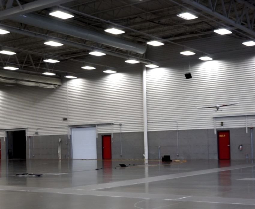
decouples the roll from the coning angle by minimising the rolling moment caused by the4.3. SIMULATION MODEL 17 misalignment of the tether tension vector and the center of mass. Two secondary cables are added to limit the sideslip at ± 20 degrees to facilitate the aircraft takeoff and landing. The load cell is a six axis Mini45 Titanium force/torque (F/T) sensor from ATI with a sensing range of 120 N in the lateral axes and 240 N in the vertical axis with the SI- 120-6 configuration. It has a resolution of 1/30 N in the lateral axes and 7/120 N in the vertical axis. The computer is running a Labview program acquiring the load cell data at a sampling rate of 10 kHz with a National Instruments USB-6003 16 bit ADC. The data is averaged over 200 samples and sent to the ground control station (GCS) at a rate of 50 Hz via a UDP connection. The position of the aircraft is evaluated using the orientation of the force vector and the length of the tether. The position of the aircraft is calculated from the measured force vector and the known tether length. The tether is assumed to be always under tension and straight because the aircraft is tethered to the load cell anchored to the ground and is flying along circular trajectories. This assumption simplifies the calculations and allows for high-frequency real- time position tracking. The tether deformation is not significant for altitude tracking with the tether lengths used in these experiments. With a tether length of 7.5 m, the measured position can be estimated to have a lateral resolution of 4 cm and a vertical resolution of 8 cm from the load cell’s specifications. The GCS used for communication between the computer and the flight controller is MAV- Proxy running a custom module to transmit the force and position data to the aircraft using the MAVLink protocol. The force and position data is saved on-board by the flight controller. Figure 4.2a shows the experimental setup during the tests with the airplane in flight and the tether highlighted in red. Figure 4.2b shows a schematic representation of the experimental setup. 4.3 Simulation Model The objective of the dynamic model is to simulate the experimental setup for controller tuning and design space exploration. The model is divided into three sub-models : the dynamics model, the aerodynamics model and the controller model. 4.3.1 Dynamics Model The aircraft is modeled as a rigid body with 6 DoF and the reference frames follow aero- nautical standards as shown in Figure 4.3. The inertial frame N is of type north-east-down (NED) and its origin is N0 . A vehicle frame V is affixed to the rigid body of the aircraft
18                            CHAPITRE 4. MODÈLE, VALIDATION ET RÉSULTATS

                                                        Ground Control
                                                           Station                       UAV

                                                                                    Tether
                                                               Load cell

  (a) Experimental setup (highlighted tether)       (b) Schematic of the experimental setup
                   Figure 4.2 Representation of the experimental setup

and its origin is the geometric point V0 that coincides with the leading edge of the wings
and a fuselage line from the nose to the tail. Its axes are parallel to the inertial frame.

The body frame B has its origin B0 at the same point as the origin of the vehicle frame.
The body’s x axis points towards the nose, the y axis points towards the starboard wing
and the z axis points down. The orientation of the body frame relative to the vehicle
frame is defined by three consecutive rotations : a yaw angle ψ rotation around the ẑV
axis, a pitch angle θ rotation around the ŷV 0 axis and a roll angle φ rotation about the x̂V 00
axis. The aircraft’s center of mass BCM is located behind B0 . The position of the body’s
center of mass is defined relative to the inertial frame by the components x,y and z as in
Equation 4.1.

                                rBCM /NO = xx̂N + yŷN + zẑN                                (4.1)

The tether is fixed on the ground at N0 and on the aircraft at the tether attachment point
BT . The vertical component of the tether tension at the anchor NO is denoted by Fz and
is positive along −ẑN . The coning angle λ is the angle between the tether and the x-y
plane in the inertial frame.

The motor thrust vector FBMM is applied at the motor mounting point BM in the direction
of x̂B and causes a pitch down moment because it is not aligned with the body’s center of
mass. The thrust and torque of the propeller are evaluated from experimental data derived
from the wind tunnel powertrain characterization. They are given as a function of airspeed
4.3. SIMULATION MODEL 19
Figure 4.3 Diagram of the simplified airplane (B), tether, anchor, reference
frames and forces included in the dynamic model.
and throttle command as in the following equations :
FP = f (Va , δT )
(4.2)
MP = g(Va , δT )
The tether is assumed to be always under tension and straight because the aircraft is
tethered to a fixed anchor on the ground and is flying along circular trajectories indoors
in a no wind environment. The tether is modeled as a spring that exerts no force when
compressed, and its force FBT T acts upon point BT in the direction of rN0 /BT . The tether’s
force acting on BT is given by the following equation :
(k ∆L ) rN0 /BT , ∆L > 0
T T T
FBT T = (4.3)
0, ∆LT < 0
where kT is the spring constant of the tether and ∆LT is the tether length variation from
its initial length LT . Since the tether has a small diameter and is relatively short, the
aerodynamic loading and the dynamic behavior of the tether is not significant for the
purpose of this model. If we were to scale up the system or model the coupled dynamics of
a tethered aircraft and payload, a dynamic tether model based on a lumped mass model
would be required [5].
The translation and angular velocities are defined in Equations 4.4 and 4.5 and Figure 4.4
shows a representation of the velocities of the body frame.
N
vBCM = ux̂B + vŷB + wẑB (4.4)
N
ω B = px̂B + qŷB + rẑB (4.5)20 CHAPITRE 4. MODÈLE, VALIDATION ET RÉSULTATS
Figure 4.4 Body frame velocities
The state vector X contains the 12 states of the model and its components are defined in
Equation 4.6.
T
X= x y z φ θ ψ u v w p q r (4.6)
The equations of motion (EoM) are obtained to solve for the state variables and their
time-derivatives. A classic Newton-Euler approach was used, as shown in Equations 4.7
and 4.8. The EoM were generated using MotionGenesis [29] and are solved in Matlab.
N
FB = mB ∗ N aBCM (4.7)
N
MB/BCM = I B/BCM · N αB + N ω B × (I B/BCM · N ω B ) (4.8)
4.3.2 Aerodynamics Model
The aerodynamic forces and torques acting on the body are calculated using linear approxi-
mations applied at BCM . The airspeed, angle-of-attack and sideslip angle are a function
of the vehicle’s velocity : √
V a = u2 + v 2 + w 2
w
α = arctan (4.9)
u
v
β = arcsin
Va
The dimensionless stability and control derivatives were calculated using the vortex lattice
method (VLM). The AVL program was used to compute the linear stability and control
derivatives at a trimmed airspeed of 18 m/s. The results are shown in Table 4.3.
The total aerodynamic forces acting on the UAV at the center of mass are :4.3. SIMULATION MODEL 21
Tableau 4.3 Dimensionless stability and control derivatives of the Skysurfer
Pro aircraft calculated using VLM
Coefficient Value Coefficient Value Coefficient Value
C xu -0.0177 Czu -0.930 Cmu 0
C xw 0.281 Czw -5.139 Cmw -1.69
C xq -0.272 Czq -9.73 Cmq -15.4
C yv -0.206 Clv -0.0914 Cnv 0.0641
C yp 0.0103 Clp -0.459 Cnp -0.0307
C yr 0.167 Clr 0.121 Cnr -0.0583
C l δa 0 C l δr 0 C m δe 0
C n δa 0 C n δr 0
−mg sin θ CX (α) + CXq (α) 2Vc a q + CXδe (α)δe
1
FBaero
CM
= mg cos θ sin φ + ρVa2 S CY0 + CYβ β + CYp 2Vb a p + CYr 2Vb a r + CYδa δa + CYδr δr
2
mg cos θ cos φ CZ (α) + CZq (α) 2Vc a q + CZδe (α)δe
(4.10)
and the total aerodynamic torques acting on the UAV are :
h i
b C l0 + C lβ β + Clp 2Vb a p
+ Clr 2Vb a r
+ C l δa δ a + C lδ r δ r
1 2 h i
MBaero = ρVa S c Cm0 + Cmα α + Cmq 2Vc a q + Cmδe δe (4.11)
2
h i
b Cn0 + Cnβ β + Cnp 2Vb a p + Cnr 2Vb a r + Cnδa δa + Cnδr δr
where CX , CZ are the lift and drag forces along the x̂B and ẑB axes as in Equation 4.12.
The other coefficients are obtained from Table 4.3.
CX = −CD cos α + CL sin α
CZ = −CD sin α − CL cos α
(4.12)
C L = C L0 + C Lα α
CL 2
CD = CD0 +
πeA
Additional details on the aerodynamic model can be found in [30].
4.3.3 Controller Model
The controller is a full flight control system that maintains the inertial position and the
attitude of the aircraft with multiple PID control loops. The longitudinal controller is22 CHAPITRE 4. MODÈLE, VALIDATION ET RÉSULTATS
decoupled from the lateral controller. Each loop has an anti-wind-up scheme and output
saturation. The controller runs at a frequency of 50 Hz. The control inputs are the ailerons
δa , the elevator δe , the rudder δr and the throttle δT .
h iT
u = δa δe δr δT (4.13)
The longitudinal controller consists of an altitude controller and an airspeed controller.
The altitude controller uses a successive loop closure strategy with a pitch attitude hold
inner loop to hold a target altitude with the elevator. The airspeed controller uses the
throttle in an airspeed hold loop. The lateral controller uses the ailerons in a roll-attitude
hold loop. Figure 4.5 shows a schematic representation of the controller.
+ +
- PID - PID model
(a) Altitude controller
+
- PID model
(b) Roll controller
+
- PID model
(c) Airspeed controller
Figure 4.5 Schematic representation of the controller
The PID gains of the control loops were first tuned using a genetic algorithm and an ISE
fitness function on step inputs of the simulation model. Then, during the experiments,
they were heuristically fine tuned based on the observations.
4.4 Results
4.4.1 Tests description
The flight tests were done at a convention center in an indoor exhibition hall to eliminate
the effect of uncontrolled wind. To evaluate the lifting capabilities of the aircraft, multiple
flight tests were done in two tether configurations : a short tether of 7.50 m and a long
tether of 12.00 m. At each tether length, an altitude sweep was performed. It consisted of
flying from 2 to 5 m above ground in increments of 0.5 m at a target airspeed of 15 m/s
and 17 m/s.4.4. RESULTS 23
The cable attachment was successful in decoupling the bank angle of the aircraft from the
coning angle. The aircraft was able to achieve coning angles in excess of 30 degrees while
maintaining the wings level. The effect of the bank angle on the lifting capabilities was
not measured during the tests. The roll of the aircraft was stabilized at 0 degrees at each
flight.
4.4.2 Controller performance
The performance of the controller was adequate for the purpose of the tests. It was able
to stabilize the aircraft at the desired set-points as expected from the simulation results.
Figure 4.6 shows the measured altitude for a segment of autonomous flight with the short
tether at an airspeed of 17 m/s. It can be observed that the altitude oscillates within about
15 cm of the target. The noise of the airspeed sensor used in the throttle control loop caused
noticeable throttle variations even though the measurements were filtered with a weighted
moving average. The additional noise could have been caused by the aircraft flying in its
own wake. Since the airspeed plays a significant role in the longitudinal dynamics, the
throttle oscillations should be the main cause of the small altitude variations.
Figure 4.6 Measured altitude for a segment of flight with a tether of 7.5 m at
17 m/s. Target altitude increases by steps of 0.5 m.
Figure 4.7 shows the aircraft’s dynamic response to a target altitude increase of 0.50 m.
The experimental data (black) and the data from the simulation model (red) are compared
against the step input (blue). The rise time of the model follows closely the measured rise
time of the experimental aircraft. The model predicts accurately the aircraft’s longitudinal
response except for the oscillations in the experimental data since the noise of the airspeed
sensor is not simulated.24 CHAPITRE 4. MODÈLE, VALIDATION ET RÉSULTATS
Figure 4.7 Model altitude response to a target altitude increase of 0.5 m vs
measured response with a tether of 7.5 m at an airspeed of 17 m/s.
4.4.3 Lifting capabilities
The data acquired with the altitude sweeps is presented in Figure 4.8 where the vertical
lifting component Fz of the tether force at the anchor is plotted as a function of the
coning angle λ. The coning angle is used instead of the altitude because it gives a better
comparison between multiple tether lengths. The experimental lifting component of the
aircraft (asterisk) is compared to the predicted value from the simulation model (line) at
an airspeed of 15 m/s in red and 17 m/s in black.
(a) Short tether (b) Long tether
Figure 4.8 Experimental (asterisk) vs modeled (line) lifting component Fz (N)
at the anchor point in the short (a) and long (b) tether configuration at 15 m/s
(red) and 17 m/s (black).
The results show that the simulation model predicts accurately the lifting component of
the tether force at the anchor. The measured data from the short tether test shows a
slight deviation from the predicted value at 32 degrees of coning angle. Sources of error4.4. RESULTS 25
that could explain the discrepancies are the wake interaction that increases the drag at
high FZ . This effect is not accounted for in the model and increases as a function of the
aircraft’s lift in addition to the conventional induced drag.
The model can be used to evaluate the lifting capabilities of the aircraft at a wide range of
airspeed and coning angles. Figure 4.9 shows the lifting component Fz as a function of the
coning angle λ from 12 m/s to 20 m/s of airspeed. As expected, an increase of airspeed
increases the lifting component at the anchor. At an equal airspeed and coning angle,
the lifting component is higher with the short tether than with the long tether because
of the increased angular velocity of the aircraft resulting in stronger inertial effects. The
simulation data follows the curves shown in Figure 4.8. At a target airspeed of 20 m/s
and with the short tether, the power limit of the airplane is reached at about 28 degrees
of coning explaining the line ending.
(a) Short tether (b) Long tether
Figure 4.9 Simulated lifting component Fz (N) at the anchor point at multiple
airspeed in the short (a) and long (b) tether configuration.
The model can also be used to evaluate the lifting efficiency of the aircraft. Figure 4.10
shows the g/W ratio as a function of the coning angle λ from 12 m/s to 20 m/s of airs-
peed. As expected, an increase of airspeed decreases the lifting efficiency of the system by
increasing the parasitic drag. An increase of coning angle increases the lifting efficiency
by increasing the vertical component of the tether tension. The lifting efficiency is slightly
higher with the short tether at low coning angles, but the aircraft can reach higher effi-
ciencies with the long tether at high coning angles because of lower inertial effects. The
aircraft is limited to a maximum coning angle of about 40 degrees with the short tether
but can reach 50 degrees with the long tether.26 CHAPITRE 4. MODÈLE, VALIDATION ET RÉSULTATS
(a) Short tether (b) Long tether
Figure 4.10 Simulated lifting efficiency (g/W) at multiple airspeed in the short
(a) and long (b) tether configuration.
The aircraft was flown near its power limit to evaluate its performance in a high lift
situation. Figure 4.11 shows the measured lifting component Fz over a period of 60 seconds
with the short tether at a coning angle of 32 degrees and an airspeed of 18 m/s. The
measured power consumption was 320 W at 90% throttle. The aircraft was able to generate
a constant lifting force of 39 N at the anchor. This is equivalent to lifting 3.5 times its
empty weight. For comparison, a heavy-lift helicopter, the Skikorsky S-64E Skycrane, can
only lift up to 1.2 times its empty weight.
Figure 4.11 Lifting component Fz with a tether of 7.5 m at a coning angle of
32 degrees and an airspeed of 18 m/s.
4.4.4 Lifting efficiency
To compare the lifting efficiency of a tethered fixed wing UAV to other types of VTOL
aircraft, the gram-to-Watt ratio (g/W) will be used. It is a useful figure of merit typically
used to compare the efficiency of propeller and motor combinations. For this comparison,
lets define this metric as the mass of the payload in grams divided by the power required
to hover at this weight as in equation 4.14. For the tethered UAV, the payload is definedVous pouvez aussi lire