Quinze années d'oscillations de baryons - Éric Aubourg APC/Université Paris Diderot et CEA Saclay - IN2P3
←
→
Transcription du contenu de la page
Si votre navigateur ne rend pas la page correctement, lisez s'il vous plaît le contenu de la page ci-dessous
Quinze années
   d’oscillations
    de baryons
              Éric Aubourg
APC/Université Paris Diderot et CEA Saclay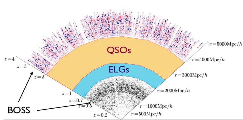
Le phénomène des oscillations de baryons

Les oscillations acoustiques de baryons (BAO,
baryon acoustic oscillations) sont devenues ces
dernières années une des méthodes d’étude de
l’énergie noire.
Elles ont la même origine que les fluctuations du
fond diffus cosmologique, mais laissent une
empreinte dans la matière, au lieu du
rayonnement électromagnétique.
Le phénomène des oscillations de baryons

Suivons l’évolution d’une surdensité adiabatique
(identique pour toutes les espèces considérées,
neutrinos, baryons, photons, matière noire — CDM)
dans le plasma primordial.
État initial

               D. Eisenstein et al. (2007)
Les neutrinos s’échappent.
La matière noire attire la matière via
la gravitation : le pic s’élargit.
Le fluide baryons+photons est
collisionnel et soumis à la pression :
onde sonore sphérique ~ 0.57 c
Découplage: les photons s’échappent
La vitesse du son diminue
Les photons se sont échappés
La vitesse du son est nulle : le pic de baryons,
parvenu à 150 Mpc de la fluctuation
originale, est gelé.
Matière noire et baryons s’attirent via
la gravité
Maintenant
Pour chaque pic de densité des fluctuations
primordiales :
— le pic original est préservé (grâce à la matière
noire !)
— on retrouve une surdensité de matière sur une
coquille située à ~150 Mpc (mesuré par CMB).

Dans l’univers plus récent, on devrait donc
observer un pic dans la fonction de corrélation des
fluctuations de matière, à une séparation de 150
Mpc.
Contraste très exagéré !
Le phénomène des oscillations de baryons fournit
un étalon de distance de ~150 Mpc, grâce auquel
on va pouvoir mesurer l’histoire de l’expansion de
l’Univers.
Premières détections : 2005

                       SDSS: Eisenstein et al. 2005
                       2dF: Cole et al. 2005
La détection des BAO dans SDSS
–9–
1. sélectionner des galaxies
lumineuses rouges (LRG) dans le
relevé photométrique SDSS par
leur couleur.
2. prendre des spectres de
~45000 LRG avec le Fig. 4.— The g ∗ − r∗ versus r∗ − i∗ color-color diagram for galaxies with 18.5 < r∗ < 19.5 from SDSS. The
spectrographe de SDSS, pour red solid lines show the selection region for Cut I LRGs. The three lines overlaid with an arrow indicates
that the location of the line cutting across the galaxy locus is a function of r∗ apparent magnitude; fainter
galaxies must be redder to pass the cut. The displayed lines correspond to r∗ = 17.5, 18.0, and 18.5, left to
mesurer leur décalage vers le right. The blue short-dashed lines show the (magnitude-independent) selection region for Cut II LRGs. The
long-dashed line shows the locus of a passively-evolving old population as a function of redshift (appendix
rouge (redshift) donc leur B); theBaryon
bend in Acoustic
the locus occurs at z ≈ 0.40. The galaxy sample is the same as in Figure 3.5
Oscillations
distance.
post-spectroscopic cuts. These are described in § 4.1.
2.3.2. Cut II (z ! 0.4)
3. Estimer la fonction de Cut II is used to select LRGs at z > 0.4 by identifying galaxies that have left the low-redshift locus in
the g ∗ − r∗ vs. r∗ − i∗ plane. At these redshifts, we can distinguish 4000Å break strength from redshift, so
corrélation à deux points (en we can isolate intrinsically red galaxies. The difficulty is avoiding interlopers, either from z " 0.4 galaxies
that scatter up in color from the low-redshift locus or from late-type stars, which are far more numerous.
utilisant des catalogues simulés
∗
We adopt rPetro = 19.5 as our flux limit because fainter objects would not reliably yield sufficient signal-
∗
to-noise ratio in the spectra. Unfortunately, the luminosity threshold in Cut I would predict rPetro > 19.5
at the redshifts of interest in Cut II. Therefore, Cut II is simply a flux-limited sample with no attempt to
comme référence, et l’estimateur produce a fixed luminosity cut across the (narrow) range of redshift probed.
The selection imposed is
de Landy-Szalay ∗
rPetro < 19.5,
Fig. 3.— As Figure 2, but plotting∗the correlation function times
(9)
(DD-2DR+RR)/RR. s2 . This shows thecvariation
⊥ > 0.45 − (g
of the r∗ )/6,
− at
peak 20h−1 Mpc scales that is (10)
controlled by the 2
2 g ∗ −redshift
r∗ > of1.30
equality (and
+ 0.25(r∗ −hence
i∗ ). by Ωm h ). Vary- (11)
ing Ωm h alters the amount of large-to-small scale correlation, but
boosting theµlarge-scale
r ∗ ,Petro to the
psf best-fit 0.5,data points on intermediate scales. (13)
Fig. 2.— The large-scale redshift-space correlation function of theBAO photométriques : se
The Clustering of Luminous Red passer
Galaxies in thede
Sloanspectrographe
Digital Sky Survey Imaging Data 17
kmin kmax ∆20 δ σδ
2.5
Les BAO peuvent être trouvées
0.005
0.010
0.010
0.025
2.8639E-04
4.4282E-03
2.2986E+00
1.0989E+00
8.7243E-01
1.1675E-01
∆ χ2= 4.73
dans des catalogues utilisant des
0.025
0.040
0.040
0.060
2.1702E-02
5.3956E-02
8.9660E-01
9.1448E-01
8.2658E-02
5.8324E-02
2.0
∆ χ2= 6.04
redshifts photométriques (photo-z),
0.060 0.075 1.0630E-01 1.0612E+00 6.0193E-02
0.075 0.090 1.5237E-01 9.3736E-01 6.0019E-02
∆2(k)/∆2CDM(k)
6 0.090 0.130 2.3303E-01 1.0118E+00 3.2957E-02
moinscosmology,
précis,
In detail, we mais
assume Dplus
0.130
0.200
and set
(z), économes
0.200
0.300
4.4947E-01 1.0281E+00
given by the fiducial
A,fid
8.5115E-01 1.2406E+00
5.4245E-02
5.0454E-02
1.5
en temps de télescope.
Table 2. The 3D real space power spectrum (for bins B1). The
D (z) = αD
A (z). A,fid (14)
bands are step functions defined by kmin < k < kmax , the fiducial
That is, we spectrum
power fix the shape
by ∆20 ,of the
and theDestimated
A (z) to be thespectrum
power same asand
La précision ~0.05(1+z) dilue
DA,fid (z) and
errors by δmeasure the that
and σδ . Note amplitude of DA (z).matrix must be
the full covariance
used for any detailed fitting to these data, since different data
pointsClustering
are anti-correlated.
1.0
4.4. evolution of lumious galaxies
l’effet le long de
In generating la ligne
the template C dewevisée
(ℓ), :
need to make
m,zi 0.01 0.10
k (h Mpc-1)
la mesure estlinear
2-D,growthdans
rate (Eq.des
a prior assumption on the evolution of the galaxy bias of
kmin kmax ∆20 δ σδ
LGs and the 9). We consider two
extreme cases of the galaxy clustering evolution: first, we
0.007 0.013 7.6073E-04 2.0776E+00 7.1312E-01
coquilles
assume successives.
0.013 0.020 3.6199E-03 2 2
9.4449E-01
that the overall clustering, b D , does not change
0.020 0.035 1.4566E-02 9.7928E-01
with redshift, which we call as ‘con-cluster’. Second, we
2.8597E-01
8.9388E-02
Figure 22. The ratio of the measured power spectrum to the
linear CDM power spectrum for our fiducial cosmology (without
baryons). As above, the solid and dashed lines represent binnings
assume 0.035
that the0.050 3.7910E-02
bias does 7.7955E-01
not change 7.3753E-02
with redshift, which B1 and B2 respectively. Also shown is the same ratio for the
0.050 0.065 7.4435E-02 9.9163E-01 6.6288E-02
Padmanabhan et al. 2006 : 600k
we call as
in the final
‘con-bias’.
0.065 0.080
0.080best0.095
The two cases9.4425E-01
1.2342E-01
fit of α, mainly because
1.6452E-01
make little5.6484E-02
difference
the expected
9.7427E-01 true
6.3003E-02
nonlinear prescription, and the “no-wiggle” fit to the power spec-
trum. The difference in χ2 between these two models is shown for
LRG
redshift0.095
distribution
0.150 sharply
2.7896E-01peaks within ±σ2.5155E-02
9.6809E-01 zph , com- the two binnings. Also note the baryonic suppression of power on
pared to0.150
the galaxy
0.250 clustering
5.9607E-01 evolution.
1.0969E+00Note that, by
4.4514E-02 large scales, and the rise in power due to nonlinear evolution on
marginalizing
0.250 over
0.350 Bz1.1610E+00 small scales
i at each photometric redshift bin
1.1772E+00 5.1480E-02
zi , we take into account the evolution of galaxy clustering
Ho et al. 2011 : 900k LRG
across Table
different redshift
3. Same bins2 whether
as Table except for we
binsuse
B2.‘con-cluster’
and ‘con-bias’. As a default, we fix b = 2 inside Cm,zi (ℓ) lar power spectra make no use of radial information, the 3D
(i.e., ‘con-bias’, and therefore the best fit Bzi can be ap- power spectrum we obtain is a real space power spectrum on
proximately interpreted as b2 (zi ).
cf. DES (en 5.cours),
0.4 LSST
TESTING THE METHOD
small scales, avoiding the complications of nonlinear redshift
space distortions. Note that on length scales much larger
0.2 than the redshift slice thickness, redshift space distortions
∆ P/σ
0.0our fitting method to the real data, we
Before applying cannot be neglected; however, the linear approximation dis-
Fig. 4.— The red circles with error bars show a power spectrum
want to validate,
-0.2using mock catalogs, that our fitting cussed over
averaged in Sec.
20 3.1.1 willmocks
N-body be valid
for on
thethese
samescales.
line of sight. TheBAO photométriques Il est possible de faire une mesure 3D si la précision des photo-z est meilleure que σz ~ 0.003(1+z). Certains projets (PAU) tentent d’obtenir cette résolution en utilisant de nombreux (~40) filtres très étroits (~ 10 nm). Physics of the Accelerating Universe (PAU) http://www.pausurvey.org
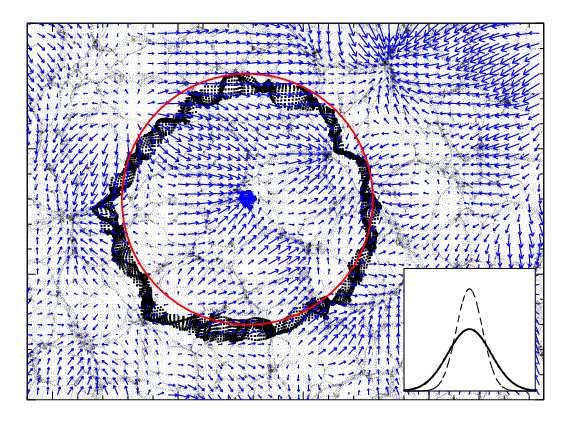
Reconstruction du régime linéaire

À bas z, les effets non linéaires deviennent importants.
Ils estompent le pic, ce qui diminue la précision de
mesure.
Il est possible d’annuler une partie de ces effets via une
« reconstruction » du régime linéaire.
Il faut reconstruire le champ de vitesse (dans le régime
linéaire) à partir de la carte des fluctuations de matière,
puis « remonter le temps » en modifiant la position des
galaxies mesurées.
Effect of non-linear clustering, from Weinberg et al. 2012
Padmanabhan et al. 2012
3 A pedagogical illustration of how reconstruction can improve the measuremen
8 Padmanabhan et al
real space redshift space
after
reco
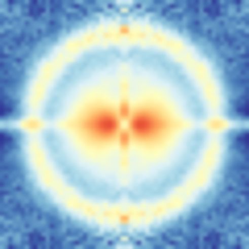
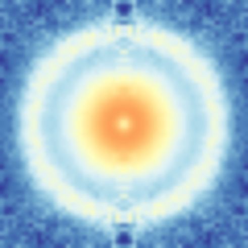
Figure 4. The LasDamas galaxy correlation function, averaged over the 160 simulations, as a function of the separation perpendicular
(?) and parallel (||) to the line of sight. The correlation functions have been scaled by r2 to highlight the BAO feature. The top panels
show the unreconstructed correlation functions, while the bottom panels show the reconstructed correlation functions; the left and right
panels are real and redshift space respectively. The BAO feature is visible as a ring at ⇠ 110Mpc/h in the top left panel. Redshift space
Padmanabhan et al. 2012
distortions destroy the isotropy of the correlation function (top right). Reconstruction both sharpens the BAO feature (highlighted inreconstructed with FOG compression
reconstructed
real space
z=0.3
z=49
Eisenstein et al. 2007presented in this paper.
he LOWZ and CMASS sam-
Analyses anisotropes
y field, applying an assumed
mate the matter density field
A correction is applied to ac- 4 MEASURING ISOTROPIC BAO POSITIONS
space distortions.
Le pic Full
BAO details
se manifeste à laposition
fois le in
long de la ligne de2-point measu
The BAO spherically averaged
ply can be found in Padman-
visée (relié à H(z)), et fixedtransversalement
by the projection (ce quisound
of the mesure
horizon at the drag
(2012). Compared to Ander-
D A(z)).
e number of points in the ran-
and provides a measure of
mating theUne displacement field, ⇥ ⇤1/3
analyse isotrope mesure DV (z) ⌘ cz(1 + z) DA (z) H (z) ,2 2 1
the shifted field (see Eisen-
Une analyse
2012; Anderson 3D compare
et al. 2012, where par nature
DA (z) is theH(z) et D
angular A(z), etdistance and H
diameter
wn that the results
inclut can be
donc unbi-test d’Alcock-Paczinsky.
Hubble parameter. Matching our DR9 analysis (Ande
ndom catalogue is too small. 2012) and previous work on SDSS-II LRGs (Percival e
e data in Il
theest
NGCnécessaire
and SGC, de prendre
we assumeen that
compte l’effet clustering
the enhanced Kaiser amplitude alon
hese two(distorsions
regions separately.
de redshift,of-sight
RSD). due to redshift-space distortions does not alter
Les RSD fournissent également de l’information sur la RAS, MNRA
c 2014
croissance des structures.Limitations intrinsèques : nombre de modes Les BAO mesurent une échelle de 150 Mpc. Dans la coquille observable dans une gamme de redshifts données, il y a un nombre fini de modes mesurables. Les BAO sont limitées par la statistique disponible, une fois données une combinaison de traceurs et de gamme de redshift.
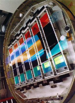
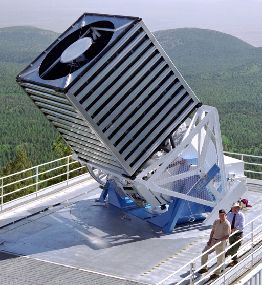
SDSS

Sloan Digital Sky Survey
(I, II, III, IV en cours)
Télescope grand champ, diamètre
2.5-m à Apache Point
Observatory, NM
Caméra d’imagerie (ugriz) de SDSS-I
(2000-2005, 8000 sq deg) et SDSS-II
(2006-2008, 10000 sq deg)
Spectroscopie SDSS

SDSS-I et II: spectrographe avec 840 fibres
SDSS-I: 675 000 galaxies, 90 000 quasars.
  Première détection des BAO dans 50 000 LRG

SDSS-II: 860 000 galaxies, 105 000 quasars
  BAO avec des photo-z, 600 000 galaxies à z~0.5
SDSS-III (BOSS), SDSS-IV (eBOSS)

Mise à niveau du spectrographe : 1000 fibres,
couverture spectrale étendue, transmission optique
améliorée.
BOSS (baryon oscillations spectroscopy survey) est un
relevé dédié à l’étude des BAO
  — dans un échantillon plus vaste de galaxies
  — dans la forêt Lyman alpha des quasars

eBOSS étend le relevé, et y ajoute des galaxies à raie
d’émission et des quasars.
SDSS,
relevé principal
SDSS,
relevé principal
SDSS-I + SDSS-II
LRG, 8000 deg2
(fin en 2008)
10-4 galaxies/Mpc3
SDSS,
relevé principal
SDSS-I + SDSS-II
LRG, 8000 deg2
(fin en 2008)
10-4 galaxies/Mpc3

SDSS-III LRG
10,000 deg2
5x densité
2x volume
BAO dans la forêt Lyman alpha

           z
          2.8                                       3.4

                         HI clouds

     La forêt Lyman-α donne accès à la densité d’hydrogène neutre le
     long de la ligne de visée d’un quasar.
     Assez de quasars : mesure 3D des BAO.
     Mesure de l’échelle BAO à z ~ 2.5 (époque non dominée par
     l’énergie noire dans les modèles classiques)
BAO dans la forêt Lyman alpha Les candidats quasars sont sélectionnés à partir de leurs couleurs (dans SDSS ou d’autres relevés), ou de leur variabilité. La sélection a une faible efficacité (mêmes couleurs que les étoiles A et F) : 30 à 50% sont vraiment des quasars. Ensuite : spectroscopie des cibles, sélection automatique et inspection visuelle pour sélectionner les quasars et déterminer leur redshift, et identifiers BAL et DLA.
Ajustement du continuum Ly-α

                                                 Lee et al. 2012

Source de distorsions dans la fonction de corrélation.
Pris en compte dans l’analyse.
ELG
Ly-α Photo-z Recons- Fourier
Phase Années MGS LRG Ly-α ELG QSO x Anisotrop RSD
-QSO BAO truction space
LRG
z 0.07 - 0.2 0.2-1.0 >2.1 >1.77 0.6-1.1 0.8-2.2 0.6-1.0
2000-2005
SDSS DR1-DR4 ✔
2005-2008
SDSS-II DR5-DR7 ✔ ✔ ✔ ✔
2008-2014
SDSS-III DR8-DR12 (✔) ✔ ✔ ✔ (✔) ✔ ✔ ✔ ✔
2014-2021
SDSS-IV DR13-DR16 ✔ ✔ ✔ ✔ ✔ ✔ ✔ ✔ ✔ ✔ ✔
(DR17 2021)observation is performed in a series of 900-second exposures, in-
tegrating until a minimum signal-to-noise ratio is achieved for the
faint galaxy targets. This ensures a homogeneous data set with a
SDSS-III sur les galaxies
high redshift completeness of more than 97 per cent over the full
survey footprint. Redshifts are extracted from the spectra using the
methods described in Bolton et al. (2012). A summary of the survey
CMASS
7e-04
DR11 LOWZ
DR11 CMASS
6e-04 DR7
Number Density (h3/Mpc3)
5e-04
313,780 BAO in SDSS-III BOSS galaxies 21
4e-04
Figure 11. DR11 CMASS clustering measurements (black circles) with ⇠(s) shown in the left panels and P (k) i
measurements prior to reconstruction and the bottom panels show the measurements after reconstruction. The solid
3e-04
690,826 case. One can see that reconstruction has sharpened the acoustic feature considerably for both ⇠(s) and P (k).
2e-04
1e-04
0.2 0.3 0.4 0.5 0.6 0.7 0.8
Redshift
Figure 1. Histograms of the galaxy number density as a function of redshift
for LOWZ (red) and CMASS (green) samples we analyse. We also display
the number density of the SDSS-II DR7 LRG sample in order to illustrate
the increase in sample size provided by BOSS LOWZ galaxies.
Figure 12. Plot of 2 vs. ↵, for reconstructed data from DR10 (blue), and DR11 (black) data, for P (k) (left) and ⇠
for a model without BAO, which we compute by setting ⌃N L ! 1 in Eqs. (23) and (26). In the ⇠(s) case, this l
2 (↵) is not constant. Our P (k) model has no dependence on ↵ in this limit. The DR11 detection significance is g
gure 15. As Figure 15, but for the DR11 LOWZ correlation function c 2014 RAS, MNRAS 000, 2–39
ansformed as defined by Eq. 46 with a = 0.39 and b = 0.04. As before,
ese error bars are nearly independent, with a worst case of 12 per cent
nd an r.m.s. of 3.4 per cent in the off-diagonal elements of the reduced
ovariance matrix.
Anderson
Figure 17. The BAO feature in the measured power spectrum et DR11
of the al. 2014measurements to the constraints they imply on ⌦m h2 , assuming the flat ⇤CDM m
scale. We stress that this inference of ⌦m h2 is entirely model-dependent and shou
an easy comparison of the CMB and BOSS data sets in the context of ⇤CDM.
SDSS-III sur les galaxies dataset ze↵ ↵ ✏
Planck BAO
0.32 in1.040
SDSS-III
± 0.016 BOSS galaxi
0.0033 ± 0.0013
WMAP 0.32 1.008 ± 0.029 0.0007 ± 0.0021
eWMAP 0.32 0.987 ± 0.023 0.0006 ± 0.0016
LOWZ 0.32 1.018 ± 0.021 -
Planck 0.57 1.031 ± 0.013 0.0053 ± 0.0020
WMAP 0.57 1.006 ± 0.023 0.0012 ± 0.0034
eWMAP 0.57 0.988 ± 0.019 0.0010 ± 0.0027
CMASS-iso 0.57 1.0144 ± 0.0098 -
CMASS 0.57 1.019 ± 0.010 0.025 ± 0.014
Figure 21. The distance-redshift relation from the BAO method on galaxy Figure 22. The DV (z)/rd measured from galaxy surveys
surveys. This plot shows DV (z)(rs,fid /rd ) versus z from the DR11 the best-fit flat ⇤CDM prediction from the Planck data. A
CMASS and LOWZ consensus values from this paper, along with those are 1 . The Planck prediction is a horizontal line at unity,
from the acoustic peak detection from the 6dFGS (Beutler et al. 2011) and tion. The dashed line shows the best-fit flat ⇤CDM predict
WiggleZ survey (Blake et al. 2011; Kazin et al. 2014). The grey region WMAP+SPT/ACT results, including their smaller-scale CMB
shows the 1 prediction for DV (z) from the Planck 2013 results, assum- (Bennett et al. 2013). In both cases, the grey region shows t
ing flat ⇤CDM and using the Planck data without lensing combined with tion in the predictions for DV (z) (at a particular redshift, a
smaller-scale CMB observations and WMAP polarization (Planck Collab- the whole redshift range), which are dominated by uncertainti
oration 2013b). One can see the superb agreement in these cosmological As the value of ⌦m h2 varies, the prediction will move coh
measurements. down, with amplitude indicated by the grey region. One can
tension between the two sets of CMB results, as discussed inSDSS-III sur
BAOles galaxiesBOSS galaxies
in SDSS-III 351.00
αi
0.95
0.90
SDSS-III sur la forêt Lyman-α
0 5 10 15
realization # N.G. Busca et al.: BAO in the Lyα fo
0.1 < µ < 0.5 F
Première détection : Busca et al. 2013
Fig. 17. The measurements of αiso (= αt = αr ) for the 15 sets of 0.8 found
mock spectra and for the data (realization=-1). The large errors 0.6 from
9 also
for realization 5 and 8 are due to the very low significance of the
48,640 QSO 2.1SDSS-III sur la forêt Lyman-α
N.G. Busca et al.: BAO in the Lyα forest of BOSS
University of Cambr
the French Participa
H(z)/(1+z) (km/sec/Mpc)
University, the Instit
90 Dame/JINA Participa
National Laboratory
Institute for Extrater
University, Ohio Sta
80 Portsmouth, Princeto
of Tokyo, University
University of Washin
70
Appendix A: M
60 We have produc
procedure and to
effects in the mea
50 In some ga
0 1 2 (2012)) the cova
z tion is obtained f
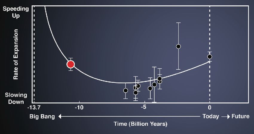
Fig. 21. Measurements of H(z)/(1+z) vs z demonstrating the ac- have very realisti
celeration of the expansion for z < 0.8 and deceleration for z > In order to doSDSS-III sur la forêt Lyman-α
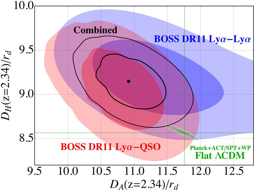
T. Delubac et al.: BAO in the Ly↵ forest of BOSS quasars

                         SDSS-III sur la forêt Lyman-α
    not be expected to be cor-
 rs. The tests with the mock                                                                             T. Delubac et al.: BAO in the Ly↵ forest of BOSS quasars
pectral diversity confirm that
stimates do not introduce bi-
peak positions.
            DR11: Delubac et al. 2014
 ibration are potentially more
h (Smee et al., 2013) is cali-

  nspectra
            158,401 QSO 2.1
SDSS-III sur QSO x Lyman-α
Cross-corrélation entre QSO et forêt Lyman-α
Font-Ribeira et al. 2014
164 017 QSO comme traceurs, 130 820 pour Lyman-α.
Plus de corrélations parasites dues au continuum.
Figure 6: Contours of 2 = 2.27 and 5.99, corresponding to Gaussian confiden
of 68% and 95%, from the Ly↵ auto-correlation analysis from DR9 ([18], in blu
SDSS-III/BOSS
Figure 1: Left panel: Redshift distribution of the 164,017 finalused
quasars papers
as2015
dens
the cross-correlation from DR11 (this work, in red) and from the joint analysis (in
The green contours show the 68% and 95% contours for the regions of this parametSDSS-III : combinaison
Combinaison des galaxies, Ly-α auto et cross-corrélation
10
30
6dFGS
MGS
SDSS II
WiggleZ
LOWZ
distance/rd z
p
20 CMASS
Ly auto
Ly cross
p
DM (z)/rd z
10 p
DV (z)/rd z
p
zDH (z)/rd z
0.1 0.2 0.5 1.0 2.0
z
Figure 1. The BAO “Hubble diagram” from a world collection of detections. Blue, red, and green points show BAO mea-
surements of DV /rd , DM /rd , and zDH /rd , respectively, from the sources indicated in the legend. These can be comparedSDSS-III : cosmologie
Les BAO seuls prouvent l’existence de l’énergie noire
Figure 4
from gala
Combined BAO (échelle BAO = paramètre libre)
1.2 tion of th
Combined BAO+Planck DM
physics t
1.0 no CMB
and 99.7
0.8 “donut”
dent con
⌦
0.6
CMB cha
0.4
0.2 meaning
BAO alo
0.0 non-zero
0.0 0.1 0.2 0.3 0.4 0.5
⌦m rameter.
ther me
compatiSDSS-III H0, inverse distance ladder
13
host galaxies of SNIa,
vailable secondary dis-
computed in absolute
cs, the combination of
ment of H0 via an “in-
intermediate redshift.
olute values of DV at
with precision of 2.0%
NIa sample provides a
le, which transfers the
redshift, where H0 is
dshift relation. Equiv-
he absolute magnitude
instead of the Cepheid
polation from the BAO
s on the dark energy
scale is precisely mea-
nterval which includes Figure 5. Determination of H0 by the “inverse dis-
ation introduces prac- tance ladder” combining BAO absolute distance measure-
e dark energy model is ments and SNIa relative distance measurements, with CMB
er the inverse distance data used to calibrate the sound horizon scale rd . The quan-
of !m and !b and thus tity c ln(1 + z)/DM (z) converges to H0 at z = 0. Filled
circles show the four BAO measurements, normalized with–8–
SDSS-IV & eBOSS
Fig. 4.— Left: eBOSS redshift coverage. eBOSS will be the first large-scale structure
Résultat publiés été 2020
expansion of the Universe in the critical range 0.8 < z < 2.2. Right: Fractional const
projected for all BAO surveys to be completed this decade.
4. eBOSS: Precision studies of dark energy and dark matte25 SDSS MGS
BOSS Galaxy
expansionhistory
eBOSS LRG
20 eBOSS ELG
eBOSS QSO
eBOSS Ly Ly
15 eBOSS Ly QSO
10
l an c k p
P DM (z)/rd z
p
zDH (z)/rd z
0.7 f 8
0.6
growth
0.5
Planck
0.4
0.3
0.2
0.1 0.2 0.5 1.0 2.0 3.0
redshift
SDSS-IV/eBOSS final papers 2020
nce measurements from the SDSS lineage of BAO measurements presented as a function o1.0
o CDM
0.5
CMB T&P
SN
BAO
o CDM
0.0 0.00
0.0 0.2 0.4 0.6 0.8 1.0
m
3.— Cosmological constraints under the assumption of a model with a w = 1 cosmological constant with
k
Table 4). Left: 68% and 95% constraints on ⌦m –⌦⇤ from the Planck CMB temperature and polarizatio
0.05 (blue). The dashed line represents a model with zero c
a sample (red), and SDSS BAO-only measurements
⌦k constraints for the combination of CMB (gray), CMB + SN (red), and CMB + BAO (blue).
CMB T&P
CMB T&P+SN
0.10 CMB T&P+BAO
0.2 0.3 0.4 0.5 0.6
mCMB T&P
0.5 SN
BAO
1.0
w
1.5
wCDM
(flat)
0.0 0.2 0.4 0.6
m
Fig. 4.— Constraints on the wCDM and ⌫⇤CDM models, as in Table 4. Le
wCDM cosmology from the Planck
P CMB temperature and polarization data (gra
measurements (blue). Right: m⌫ –⌦m constraints under the assumption of aRSD : redshift space distorsions
Cosmology from eBOSS 2
Ωk = -0.044 w = -1.58 Σmν = 0.268eV Ωm = 1
Fig. 7.— The SDSS f 8 measurements as a function of redshift, normalized by the Planck 2018 bestfit ⇤CDM model (shown in dotte
black). The three colored curves represent the fractional deviations
P from ⇤CDM for an o⇤CDM model with ⌦k = 0.044 (red), a wCDM
model with w = 1.58 (green), and a ⌫⇤CDM model with m⌫ = 0.268 eV (blue). These are the same models as those in Figure 2. A
Einstein de Sitter model (magenta; ⌦m = 1, ⌦⇤ = 0 and 8 (z = 0) matching that of fiducial model) is ruled out at high confidence, furthe
demonstrating the long-standing preference for growth measurements for models with lower matter densities.
TABLE 6
Marginalized values and 68% confidence limits on curvature, dark energy parameters, and the amplitude of density fluctuations.
⌦m ⌦DE 8 ⌦k w
CMB T&P 0.483+0.055
0.069 0.561+0.050
0.041
+0.016
0.774 0.014 0.044+0.019
0.014
+0.052 +0.045 +0.017
CMB T&P + RSD 0.455 0.581 0.780 ± 0.014 0.036Cosmology from eBOSS 29
Stage III
Stage III w/o SDSS
Stage II + SDSS
Stage II
0.285 0.300 0.315 0.68 0.70 0.000 0.008 0.016
m k
0.72 0.80 67.5 69.0 70.5 1.08 1.02 0.96 0.0 0.5 1.0
8 H0 w0 m⌫ [eV]
4.— Central values and 68% contours for each of the parameters describing expansion history and growth of structure in a ⌫owCDM
Results are shown for each data set combination presented in the text, where Stage-II corresponds to a combination of the WMAP,
nd SDSS DR7 data and Stage-III corresponds to a combination of the SDSS BAO+RSD, Planck, Pantheon SN Ia, and DES 3⇥2pt
= |Cov(p, p)| 1/(2N ) , where N = 5 is the number value for the power-law index of the primordial power
parameters (represented by p). This form prop- spectrum. The model that best describes the Ly↵ and
acks the typical gain in the 68% confidence interval Planck data has a running that is non-zero at more than
h free parameter. We find FoM = 11, 23, and 44 95% confidence, ↵s ⌘ dns /d ln k = 0.010 ± 0.004.
e Stage-II, Stage-II+SDSS, and Stage-III results, The eBOSS data have been used to further explore
tively. The gain by a factor of 2 when adding the inflationary models through tests for primordial non-technique (SH0ES, Riess et al. 2019).
TABLE 5
Hubble parameter constraints.
Dataset Cosmological model H0 (km s 1 Mpc 1 ) Comments
CMB T&P+BAO+SN ow0 wa CDM 67.87 ± 0.86 Inverse distance ladder
BBN+BAO ⇤CDM 67.35 ± 0.97 No CMB anisotropies
CMB T&P ⇤CDM 67.28 ± 0.61 Planck 2018 (a)
+3.3
CMB T&P o⇤CDM 54.5 3.9 Planck 2018 (a)
Lensing time delays ⇤CDM 73.3 ± 1.8 H0LiCOW (b)
Distance ladder - 74.0 ± 1.4 SH0ES (c)
GW sirens - 70 ± 10 LIGO (d)
TRGB - 69.6 ± 1.9 LMC anchor (e)
TFR - 76.2 ± 4.3 Cosmicflows (f)
Note. — The top section shows constraints derived in this paper, while the bottom section shows a compilation of results
from the literature: (a) CMB anisotropies measured by the Planck satellite (Planck Collaboration et al. 2018b); (b) time delays
from six gravitationally lensed quasars from H0LiCOW (Wong et al. 2020); (c) distance ladder with Cepheids and SNe Ia from
the SH0ES collaboration (Riess et al. 2019); (d) gravitational wave detection of a neutron star binary merger by LIGO (Abbott
et al. 2017a); (e) tip of the red giant branch (TRGB) calibrated with the LMC distance (Freedman et al. 2020); (f) Tully-Fisher
relation (TFR) from the Cosmicflows database of galaxy distances (Tully et al. 2016).
olate the constraints to redshift zero. One example of this BAO measurements allow estimates of H0 that are ro-
indirect measurement is that obtained using time delays bust against the strict assumptions of the CMB-only
in strongly-lensed quasars (e.g., Birrer et al. 2019). Other estimates. First, we combine Planck temperature and
indirect measurements of H0 use CMB data under strong polarization, SN, and BAO data and allow a very flexi-
assumptions about the model governing the expansion ble expansion history to demonstrate that the tension in
history from the last scattering surface to today. The H0 estimates is not due to the assumptions of a ⇤CDM
CMB estimates typically give considerably lower values model. Second, we present a measurement of H0 that
of the Hubble constant. The final Planck data release, for uses BAO and a BBN prior that is independent of CMB
example, finds H0 = 67.36 ± 0.54 km s 1 Mpc 1 (Planck anisotropies to demonstrate that the tension is not due
Collaboration et al. 2018b) when assuming the ⇤CDM to systematic errors in the CMB data. We finish this sec-
model. tion presenting the combination of the BAO data with
Explanations for the tension between direct measure- the local distance ladder measurement, and we discuss
ments and CMB estimates range from underestimated the low value of rd inferred from this analysis.
systematic errors or modeling of the primordial power
spectrum (e.g., Davis et al. 2019; Dhawan et al. 2020; 4.2.1. H0 and the inverse distance ladder
Anderson 2019; Hazra et al. 2019), to models for dark
energy (e.g., Li & Shafieloo 2019; Alestas et al. 2020; Di In this subsection we present a cosmological measure-
Valentino et al. 2020), to unmodeled pre-recombination ment of H0 without an assumption of a flat ⇤CDM
physics that lead to a decreased sound horizon scale (e.g., model. This approach is often referred as the inverse
Poulin et al. 2019; Chiang & Slosar 2018; Beradze & Gog- distance ladder, as it relies on a calibrated distance mea-
berashvili 2020; Vagnozzi 2019; Lin et al. 2019; Arendse sure at high redshift that is then extrapolated to z = 0.
et al. 2019). See Knox & Millea (2020) for a review of Schematically, we use information from the CMB to cal-
possible solutions to the tension. ibrate the BAO distances. Those in turn are used to
We provide here two alternative analyses to show how calibrate the absolute luminosity of SNe Ia.
Since the BAO feature follows DH (z)/rd = c/H(z)/rdfrom eBOSS 19
180
CDM Distance Ladder
Sound horizon at drag epoch
160
rd [Mpc]
140 BAO
BAO+BBN
BAO+Distance Ladder
CMB T&P
120
60 65 70 75 80
H0 [km/s/Mpc]
Fig. 6.— Cosmological constraints on H0 and rd under the as-The Hubble Hunter’s Guide⇤
L. Knox† and M. Millea‡
(Dated: September 18, 2019)
Measurements of the Hubble constant, and more generally measurements of the expansion rate and
distances over the interval 0 < z < 1, appear to be inconsistent with the predictions of the standard
cosmological model (⇤CDM) given observations of cosmic microwave background temperature and
polarization anisotropies. Here we consider a variety of types of departures from ⇤CDM that could,
in principle, restore concordance among these datasets, and we explain why we find almost all of them
unlikely to be successful. We single out the set of solutions that increase the expansion rate in the
decade of scale factor expansion just prior to recombination as the least unlikely. These solutions
are themselves tightly constrained by their impact on photon di↵usion and on the gravitational
driving of acoustic oscillations of the modes that begin oscillating during this epoch – modes that
project on to angular scales that are very well measured. We point out that a general feature of
such solutions is a residual to fits to ⇤CDM, like the one observed in Planck power spectra. This
residual drives the modestly significant inferences of angular-scale dependence to the matter density
and anomalously high lensing power, puzzling aspects of a data set that is otherwise extremely well
fit by ⇤CDM.
I. INTRODUCTION determined sound horizon and showed that it is low
than the ⇤CDM Planck-determined sound horizon
Estimates of the Hubble constant from a distance 7%, amounting to a 2.6 di↵erence.
der approach are generally higher than those de- Aylor et al. [13, hereafter A19] repeated this analy
ed from cosmic microwave background (CMB) data, with updated data, and found the sound horizon tens
arXiv:1908.03663
uming the standard “⇤CDM” cosmological model to be robust to choice of CMB dataset, and thereby
The SH0 ES team calibrates a supernova sample gued against systematic errors in CMB data as a souDark Energy Survey Blanco Telescope (4 m) à Cerro Tololo au Chili 520 Mpix DECam camera Relevé en cours depuis mi-2013 BAO avec photo-z (Δz ~0.08), 300 M galaxies z
LSST
Télescope de 8,4 m à Cerro Pachon au Chili
Caméra de 3 milliards de pixels
Photo-z BAOChapter 15: Cosmological Physics
Début du relevé en 2022 (?)
PFS (Sumire) at Subaru
Prime Focus Spectrograph (PFS) : spectrographe à 2400
fibres, au foyer du Subaru, télescope grand champ de
8,2 m à Hawaii.
BAO spectroscopiques, sur 1400 degrés carrés, 4 M
galaxies, 0.8 < z < 2.4.

Synergie prévue
avec HSC
(HyperSuprime
Camera), camera
d’imagerie
actuellement au
Subaru.
DESI

Dark Energy Spectroscopic Instrument
Télescope de 4 m NOAO Mayall (Kitt Peak, AZ)
30M gal (bright, LRG, ELG) +qso, 700k Ly-α, 14000
degrés carrés
Commissioning
terminé
Euclid

Télescope spatial de 1,2 m, au point de Lagrange
Terre-Soleil L2. Champ de 0,5 degré carré.
Relevé en 2022.
Imagerie visible (lentilles gravitationnelles), imagerie
infrarouge (photo-z), spectrographie sans fente dans le
proche infrarouge (BAO).
50 M gal (Hα), 0.7 < z < 2.1
SKA (Square kilometer array)
                 Relevé radio à 21 cm, 202x, Afrique du Sud et Australie.
                 BAO avec ~ 1 milliard de galaxies, ou bien via la mesure
                 de l’intensité de l’émission de l’hydrogène.
Measuring BAO with future SKA surveys               Philip Bull

                                           Measuring BAO with future SKA surveys                                                           Philip Bu

                                           Figure 4: Forecast constraints on (w0 , wa ) for several SKA configurations and Euclid, in combination wi
                                           Planck and BOSS. All other parameters have been marginalised, including WK , and the bias is free per z bi
Au-delà des BAO La méthode des BAO atteint ses limites statistiques avec les relevés prévus (DESI, Euclid, SKA). Les relevés de matière 3D permettent d’autres analyses : — distorsions de redshift (RSD) : croissance des structures. — champs de vitesse via reconstruction, corrélation avec effet SZ cinétique. — corrélation avec effet de lentille sur objets d’arrière- plan et CMB.
Vous pouvez aussi lire