Velocity of climate change
can inform protected areas
planning and biodiversity
conservation in Ontario
←
→
Transcription du contenu de la page
Si votre navigateur ne rend pas la page correctement, lisez s'il vous plaît le contenu de la page ci-dessous
Velocity of climate change can inform protected areas planning and biodiversity conservation in Ontario

Velocity of climate change can inform
protected areas planning and biodiversity
conservation in Ontario

  L.F.G. Gutowsky and C. Chu

  Aquatic Research and Monitoring Section, 2140 East Bank Drive,
  Peterborough, ON K9L 0G2

  2019

                       Science and Research Branch
             Ontario Ministry of Natural Resources and Forestry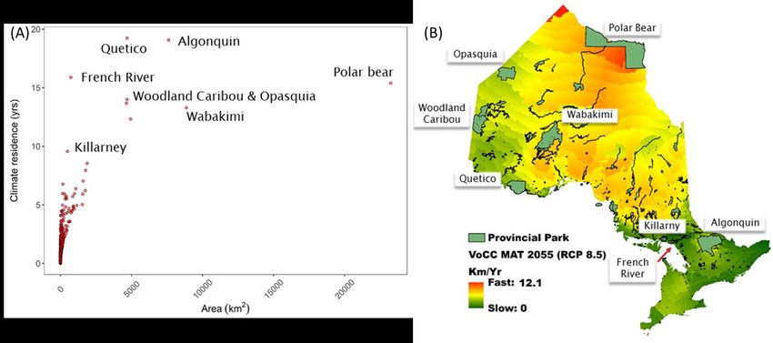
© 2019, Queen’s Printer for Ontario
Printed in Ontario, Canada

Single copies of this publication are available from info.mnrfscience@ontario.ca.

Cette publication hautement spécialisée, Velocity of Climate Change Can Inform
Protected Areas Planning and Biodiversity Conservation in Ontario, n’est disponible
qu’en anglais en vertu du Règlement 671/92 qui en exempte l’application de la Loi sur
les services en français. Pour obtenir de l’aide en français, veuillez communiquer avec
le ministère des Richesses naturelles au info.mnrfscience@ontario.ca.

Cover: clockwise from top: Nagagamisis Provincial Park and surrounding protected
areas in relation to the velocity of climate change in growing degree days >5 °C; climate
normal conditions for mean annual temperature were calculated from 1981 to 2010;
projected mean annual temperature was calculated using an ensemble mean global
circulation model under the RCP 8.5 greenhouse gas emissions scenario to 2085. View
of Smoke and Behan Lakes in Algonquin Provincial Park. A science and research team
in Quetico Provincial Park.

Some of the information in this document may not be compatible with assistive
technologies. If you need any of the information in an alternate format, please contact
info.mnrfscience@ontario.ca.

Cite this report as:
       Gutowsky, L.F.G. and C. Chu. 2019. Velocity of climate change can inform
       protected areas planning and biodiversity conservation in Ontario. Ontario
       Ministry of Natural Resources and Forestry, Science and Research Branch,
       Peterborough, ON. Climate Change Research Report CCRR-51. 34 p. +
       appendix.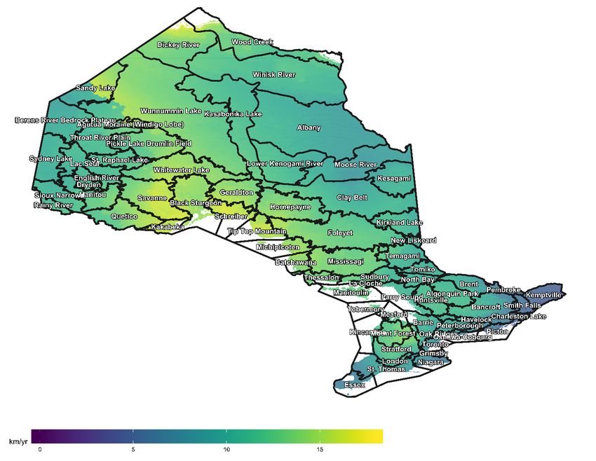
Abstract
     Climate change is a major threat to the integrity of Earth’s ecosystems. Protected
areas such as parks and conservation reserves are established to preserve the diversity
of natural features and to protect against anthropogenic stressors, which in the 21st
century includes climate change. Assessing the buffering capacity and resilience of
these protected places has become a high priority as environmental conditions and
species ranges shift in response to a changing climate. The velocity of climate change
(VoCC), defined as the instantaneous pace (km·yr-1) of climate change, is a versatile
tool to quantify how climate is changing in space and time. Here, we discuss how two
metrics associated with VoCC, exposure and climate residence time, can be used to 1)
inform the selection of new protected areas, 2) guide management planning in existing
areas, and 3) identify potential refugia in protected areas. In Ontario, ecodistricts are the
first spatial unit for selecting protected areas. Using the Bancroft Ecodistrict, specifically
the Moira River area and surrounding Crown lands, we illustrate how velocity of climate
change can be used with Ontario’s existing gap analysis tool to select potential sites for
new protected areas. Expectations are that new or existing protected areas in
ecodistricts with low exposure to climate change are less likely to be affected than those
in ecodistricts with high exposure. In high exposure ecodistricts, management planning
for existing protected areas should include climate change adaptation actions. We also
demonstrate how exposure can be used to determine the vulnerability to climate change
of brook trout lakes in Algonquin Provincial Park. Relative climate residence times were
calculated for several northern Ontario parks to demonstrate that large protected areas
with complex topographies may offer microclimates and refugia that buffer the effects of
climate change. Knowing the pace of climate change in new and existing protected
areas will improve the management planning process and inform broader biodiversity
conservation efforts.

Résumé
La vitesse du changement climatique peut éclairer la planification des aires
protégées et la conservation de la biodiversité en Ontario

    Le changement climatique représente une grave menace pour l’intégrité des
écosystèmes de la Terre. Des aires protégées, tels les parcs et les réserves de
conservation, sont établies pour préserver la diversité des caractéristiques naturelles et
pour contrer les facteurs de stress anthropiques, qui, au 21e siècle, incluent le
changement climatique. Évaluer le pouvoir tampon et la résilience de ces lieux protégés
est désormais une grande priorité face à la transition des conditions environnementales

Climate Change Research Report CCRR-51                                                      v
et des aires de répartition des espèces en réaction au changement climatique. La
vitesse du changement climatique (VCC), définie comme le rythme instantané (km·an-1)
du changement climatique, est un outil polyvalent pour quantifier l’évolution du climat
dans l’espace et dans le temps. Nous analysons ici la façon dont deux mesures liées à
la VCC, l’exposition et le temps de résidence, peuvent servir à 1) éclairer la sélection de
nouvelles aires protégées, 2) guider la planification de la gestion dans certains secteurs
et 3) repérer d’éventuels refuges dans les aires protégées. En Ontario, les écodisctricts
constituent la première unité spatiale pour la sélection d’aires protégées. À partir de
l’exemple fourni par l’écodistrict de Bancroft, plus particulièrement le secteur de la
rivière Moira et le territoire de la Couronne environnant, nous illustrons comment la
vitesse du changement climatique peut être combinée avec l’outil existant de l’Ontario
pour l’analyse de l’écart afin de sélectionner des sites susceptibles de devenir de
nouvelles aires protégées. Il est vraisemblable que les aires protégées nouvelles ou
existantes dans les écodistricts peu exposés au changement climatique soient moins
enclines à subir des répercussions que les autres. Dans les écodistricts très exposés, la
planification de la gestion des aires protégées existantes devrait inclure des mesures
d’adaptation au changement climatique. Nous montrons également comment
l’exposition peut servir à déterminer la vulnérabilité au changement climatique des lacs
d’omble de fontaine dans le parc provincial Algonquin. Le temps de résidence par
rapport au climat est calculé pour plusieurs parcs du Nord de l’Ontario afin de
démontrer que les grandes aires protégées aux topographies complexes peuvent offrir
des microclimats et des refuges qui amortissent les effets du changement climatique.
Le fait de connaître le rythme du changement climatique dans des aires protégées
nouvelles et existantes améliorera le processus de planification de la gestion et guidera
les efforts de conservation plus vastes de la biodiversité.

Acknowledgements
    Thanks to Trevor Middel, MNRF, for supplying brook trout spatial data and to
Shannon Fera, MNRF, for sharing literature and her expertise. We are grateful to Jenny
Gleeson, Josh Cornfield, Anurani Persaud, Karen Hartley, Louis Chora, David Webster,
all with MNRF, and the Priorities and Planning Section of MNRF's Climate Change
Fund, 2017-18 to 2019-20, and Protected Areas Section for funding this work.

Climate Change Research Report CCRR-51                                                   vi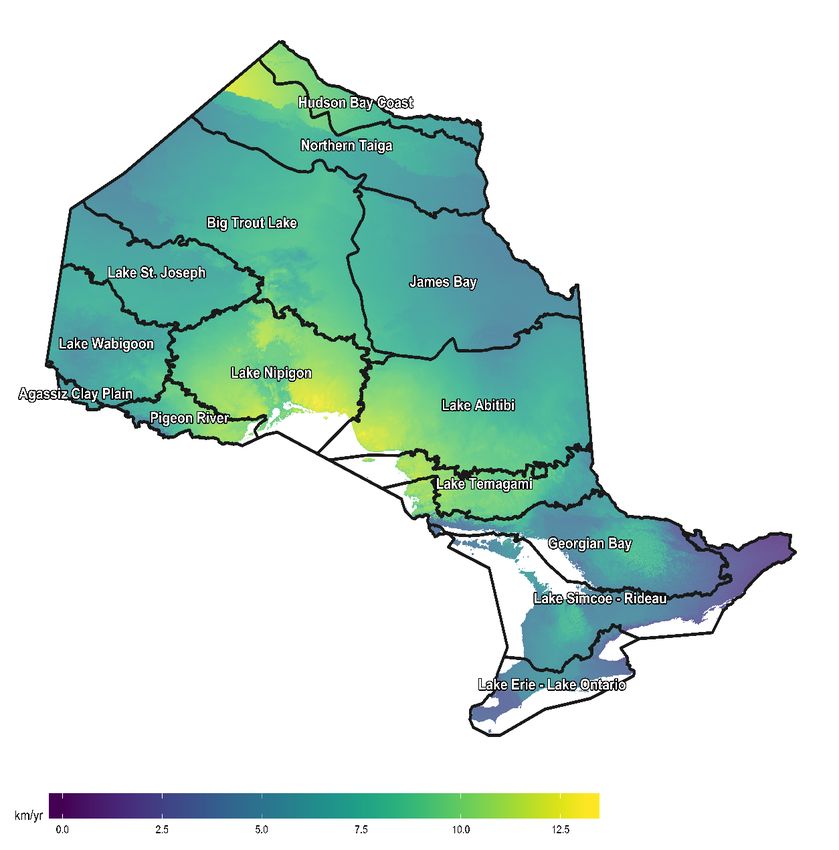
Contents
  Abstract ....................................................................................................................... v
  Résumé ....................................................................................................................... v
  Acknowledgements......................................................................................................vi
  1.0 Introduction ............................................................................................................ 1
  2.0 Velocity of climate change methods ...................................................................... 3
        2.1 Velocity of climate change uncertainty ........................................................... 4
  3.0 Calculating velocity of climate change for Ontario ................................................. 5
        3.1 Summary of projected temperature and growing degree days in Ontario ....... 5
  4.0 Considering climate change in selecting protected areas to support
      biodiversity conservation........................................................................................ 9
  5.0 Velocity of climate change applications ............................................................... 10
        5.1 Exposure to climate change in relation to Ontario’s ecological land
           classification hierarchy .................................................................................. 10
        5.2 Exposure and selecting new protected areas ............................................... 15
        5.3 Exposure and existing protected areas ........................................................ 18
        5.4 Exposure, refugia, and underrepresented habitats ....................................... 19
        5.5 Climate residence times ............................................................................... 23
        5.6 Climate residence times and existing protected areas ................................. 26
        5.7 Climate residence times, habitat, and refugia ............................................... 27
  6.0 Conclusions ......................................................................................................... 28
  7.0 Literature cited ..................................................................................................... 30
  Appendix 1. Glossary................................................................................................. 35

Climate Change Research Report CCRR-51                                                                                          vii
Climate Change Research Report CCRR-51 viii
1.0 Introduction
    Climate change is a major threat to the integrity of Earth’s ecosystems. The effect of
climate change is highest in northern regions—such as Canada—where diverse
ecosystems exist across an expansive latitudinal distance. In fact, loss of snow and sea
ice in the north (known as Arctic amplification) means that Canada is warming twice as
quickly as the rest of the world (Flato et al. 2019). Both the Intergovernmental Panel on
Climate Change (IPCC) summary for policy makers (IPCC 2018) and a synthesis of
effects for Canada (Flato et al. 2019) indicated that between 2030 and 2052 global
warming is likely to reach 1.5 °C above pre-industrial levels. These changes may cause
long-lasting or irreversible effects such as the loss of ecosystems and species (IPCC
2018).

    Methods for assessing climate change effects have been broadly categorized into
local and regional metrics (Garcia et al. 2014). Local metrics are used to compare site-
specific, historic data (e.g., tree rings, corals, ice cores, or historical records) to
contemporary conditions and climate anomalies (departures from a normal climate such
as El Niño events) (IPCC 2001). Regional metrics are used to examine how the
emergence of new or the disappearance of current climate conditions in time and space
are related to habitats, species, and ecosystems across landscapes (e.g., Williams et al.
2007, Zhu et al. 2012). The local, temporal approach helps determine how species
demographics or seasonal reproductive timing are affected by climate (Williams et al.
2007, Sunday et al. 2010, Jiménez et al. 2011), whereas the regional approach is useful
to understand species distributions and dispersal (Jackson and Overpeck 2000,
VanDerWal et al. 2013, Willis et al. 2013). While both local and regional metrics have
furthered understanding of the effects of climate change (Garcia et al. 2014), regional
shifts have recently been highlighted for their utility in addressing conservation needs
for protected areas (e.g., Chen et al. 2016, Carroll et al. 2017).

    In Ontario, the Provincial Parks and Conservation Reserves Act (Statutes of Ontario
2006) was implemented to permanently protect ecosystems that are representative of
Ontario’s natural diversity (OMNR 2011). Protected areas are designated spaces in the
public domain where resource extraction and land use restrictions contribute to the
protection of natural systems (Soares-Filho et al. 2010). Because the boundaries of
protected areas, such as parks and conservation reserves, are static, shifting climatic
conditions may limit the effectiveness of intended permanent protections (Alagador et
al. 2014, D’Aloia et al. 2019). Nevertheless, protected areas continue to be one of the
best defenses against human-caused environmental stressors (Thomas and Gillingham
2015).

Climate Change Research Report CCRR-51                                                   1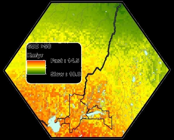
Given our current understanding of climate change, the expansion of existing or
designation of new protected areas can benefit from a regional assessment of climate-
related parameters and the historic or anticipated reactions of recipient ecological
communities (Parrish et al. 2003, Pyke and Fischer 2005, Heller and Zavaleta 2009).
Loarie et al. (2009) developed a novel index, the velocity of climate change (VoCC) or
climate velocity, to identify at risk ecosystems at global scale. VoCC is an estimate of
the instantaneous rate (km·yr-1) at which climate conditions are changing. It is thought
of as the pace needed to achieve the same historic or current climatic conditions
somewhere on the landscape under a future climate scenario. In the assessment by
Loarie et al. (2009), only a fraction of small protected areas in temperate regions had
climate residence times (estimate of years for climate to change) exceeding 100 years.
They concluded that some ecosystems may require an expanded network of protected
areas to increase their resilience and conserve biodiversity, and that keeping pace with
climate change is more feasible in protected areas with relatively little fragmentation.
Since the seminal article in 2009, VoCC has become one of the most widely used tools
to estimate the movement needed for species to remain in their climatic niche (Ordonez
and Williams 2013a,b; Vanderwal et al. 2013; Hiddink et al. 2015) and to understand the
effects of climate change on ecosystems (Hamann et al. 2015, Brito-Morales et al.
2018).

                             Velocity of climate change (VoCC)
                             is an estimate of the instantaneous
                                rate (km·yr-1) at which climate
                                   conditions are changing.

    Provincial strategies support the integration of climate change adaptation
considerations into management planning for protected areas (OMNRF 2017, MECP
2018). Ontario has 340 regulated provincial parks, 295 regulated conservation reserves,
and 11 wilderness areas covering about 9.7 million hectares of lands and waters, or
about 9% of the province’s total area. The intent is to expand the network by regulating
recommended provincial parks and conservation reserves. As a tool, VoCC has many
applications that are directly relevant to the development and management of protected
areas in Ontario. Here we provide information about VoCC, including how to calculate,
interpret, and apply it. We emphasize applications related to Ontario’s ecosystems and
potential uses for it in planning and managing protected areas and supporting
biodiversity conservation.

Climate Change Research Report CCRR-51                                                2
2.0 Velocity of climate change methods
Velocity of climate change requires inputs of climate normals (e.g., a 30-year
average of a historical climate variable; ECCC 2017) and a future scenario for the same
climate variable. Future climate scenarios, often projected to 2025, 2055, or 2085, are
derived from general circulation models (GCM), an ensemble of GCMs, or downscaled
models derived from GCMs. GCMs are mathematical models of planetary atmospheric,
oceanic, and lithospheric processes. They are coupled with representative
concentration pathway (RCP) scenarios, which represent radiative forcing measured in
watts·m-2, such that each of the RCP scenarios produce different levels of heat at the
end of the century: 8.5, 6.0, 4.5, and 2.6 watts·m-2. These scenarios describe human
population size, economic activity, lifestyle, energy use, land use patterns, technology,
and climate policy to project potential future climate scenarios (IPCC 2014). The RCP
2.6 scenario represents a future in which greenhouse gas (GHG) emissions are strictly
mitigated and peak early, RCP 4.5 and 6.0 represent intermediate GHG emissions
scenarios, and RCP 8.5 represents very high GHG emissions and a failure to curb
warming by 2100.
Two basic methods are used to calculate the velocity of climate change, both based
on dividing area into gridded cells. The original index uses local or gradient-based
climates to predict velocities (Loarie et al. 2009). Velocity is derived from the ratio of
temporal and spatial gradients of some climate variable. For example, the velocity of
mean annual temperature is calculated as:
°C·yr-1 ÷ °C·km-1 = km·yr-1 [1]
where, for the focal grid cell, the change in a climate variable through time (°C·yr-1),
often derived from a regression slope, is divided by the spatial gradient (°C·km-1),
derived as a weighted sum of the latitudinal and longitudinal pairwise differences in
temperatures from the neighbouring cells, to generate the index of velocity (km·yr-1).
The estimate is local because the spatial gradient is calculated from the nearest
neighbouring cells (Brito-Morales et al. 2018).
Distance-to-analog VoCC is a modification of the original index (Ordonez and
Williams 2013b, Hamann et al. 2015, Roberts and Hamann 2016). For a given focal cell,
the process relies on an algorithm to search all cells for an analogous climate value (± a
user-specified precision, e.g., 0.1 °C; Figure 1).
ΔD ÷ ΔT = km·yr-1 [2]
where ΔD is the distance between climate analogs (km) and ΔT is the difference in time
(yrs).
Climate Change Research Report CCRR-51 3Algorithms for the distance-to-analog calculation are found in Hamann et al. (2015). A technical manual that follows this method (Gutowsky et al. 2019) was used as a guide to calculate VoCC for the protected areas in Ontario. Figure 1. Climate velocity is calculated from a climate normal grid of cells (time1) and a projected climate scenario on a grid of the same dimensions (time2), both containing climate values, e.g., mean annual air temperature in °C. Distance to analog (Dist grid) is generated from an algorithm that searches for the closest climate match based on the specified level of precision. Velocity is calculated by dividing distance by the difference in time (time2 – time1). The focal cell is outlined in red. 2.1 Velocity of climate change uncertainty While error has been modelled into a calculation of VoCC using a Bayesian framework (Schliep et al. 2015), no standard measure of uncertainty exists. The resolution of gridded data used for the GCM and the accuracy of the GCM both between time periods and among models will introduce error. Climate Change Research Report CCRR-51 4
3.0 Calculating velocity of climate change for Ontario
    The velocity of climate change grids for Ontario were calculated following the
method described by Gutowsky et al. (2019). We used ClimateNA v. 5.20 (Wang et al.
2016), which is software used to extract and downscale monthly climate normal data
and monthly solar radiation normal data from a moderate spatial resolution (4 x 4 km) to
scale-free points for specific locations based on latitude, longitude, and elevation (the
latter is optional; see Gutowsky et al. 2019). Future climate data are downscaled and
integrated from the Coupled Model Intercomparison Project phase 5 (CMIP5) database
corresponding to the fifth IPCC assessment report for future projections (IPCC 2014).
Ensemble projections are average projections from 15 CMIP5 models.

    Input points (longitude and latitude) were generated from a digital elevation model of
Ontario and the surrounding landscape (total area of ~5.5 million km2 including the
Great Lakes and Hudson Bay; Figure 2). Using our DEM (WGS84) and elevation data,
ClimateNA grids (with decimal degree dimensions) of the 1981 to 2010 climate normals
were generated for mean annual air temperature (MAT) and growing degree days
above 5 °C (GDD5). These variables were selected because they significantly influence
the function, structure, and composition of terrestrial and aquatic ecosystems. For
instance, growing degree days, the time integral of daily temperature above a threshold,
strongly predicts growth and development in fish (Neuheimer and Taggart 2007).
Projected MAT and GDD5 data were generated using ensemble mean downscaled
GCMs for 2055 and 2085 under GHG mitigation (RCP 4.5) and business as usual
scenarios (RCP 8.5).

3.1 Summary of projected temperature and growing degree
days in Ontario
   Under RCP 4.5, MAT is predicted to increase 2.6 °C and mean GDD5 above 5 °C is
predicted to increase by 487 days by 2055 (Table 1). Under RCP 4.5 predicted in 2085,
minimum MAT will increase by 3.9 °C and maximum GDD5 will increase by 711 GDD
from current climate normal conditions in Ontario (Table 1).

   Given RCP 8.5, MAT is predicted to increase 3.6 °C and mean GDD5 above 5 °C is
predicted to increase by 680 days by 2055 (Table 1). Under RCP 8.5, mean MAT and
mean GDD5 are predicted to increase 270% and 154% by 2085, respectively. Under
RCP 8.5 in 2085, minimum MAT will increase by 7 °C and maximum GDD5 will increase
by 1621 GDD from current climate normal conditions in Ontario (Table 1).

Climate Change Research Report CCRR-51                                                   5
Table 1. Summary of Ontario mean annual temperature (MAT) and growing degree
days >5 °C (GDD5) calculated from climate normals (1981–2010) and general
circulation model ensemble mean climate projection (2055 and 2085) scenarios (RCP
4.5 and RCP 8.5).
Condition Minimum First Median Mean Third Maximum
quartile quartile
MAT (1981–2010) -8.10 -1.20 2.90 3.52 8.70 15.60
GDD5 (1981–2010) 272 1127 1604 1813 2508 4113
MAT 2055 RCP 4.5 -5.20 1.40 5.60 6.11 11.3 17.50
MAT 2085 RCP 4.5 -4.20 2.20 6.30 6.83 11.8 18.10
MAT 2055 RCP 8.5 -4.00 2.50 6.60 7.12 12.0 18.40
MAT 2085 RCP 8.5 -1.10 5.20 9.00 9.53 14.10 20.30
GDD5 2055 RCP 4.5 438 1506 2100 2300 3119 4824
GDD5 2085 RCP 4.5 497 1622 2236 2434 3281 4996
GDD5 2055 RCP 8.5 537 1669 2293 2493 3341 5083
GDD5 2085 RCP 8.5 844 2122 2791 2987 3887 5734
The resultant raw data of projected climate conditions were loaded into the R
statistical environment where a nearest-neighbour search algorithm identified the
closest matching climate (e.g., within a precision of ±0.25 °C to define a climate match;
Hamann et al. 2015) for each value. These data were converted to km·yr-1 (by dividing
distance by the interim number of years between the climate normal period and the
projected year) and converted to a 1x1 km raster of MAT and GDD5 VoCC for the
province.
At a 1x1 km resolution, Ontario VoCC rasters were generated as grids of 988,024
cells projected in Lambert conformal conic. The fastest median velocities occurred
under the RCP 8.5 business as usual scenarios predicted in 2055 (Table 2). Despite
calculating VoCC for an area about five times the size of Ontario (Figure 2), no-analog
velocities were present for three of the four variable-year combinations where GHG
emissions were business as usual (RCP 8.5) (Table 2). No-analog velocities occur
when climatic equivalents are not present in the future, e.g., under the business as
usual GHG emissions scenario, the cool MAT along Hudson Bay may no longer exist by
2085.
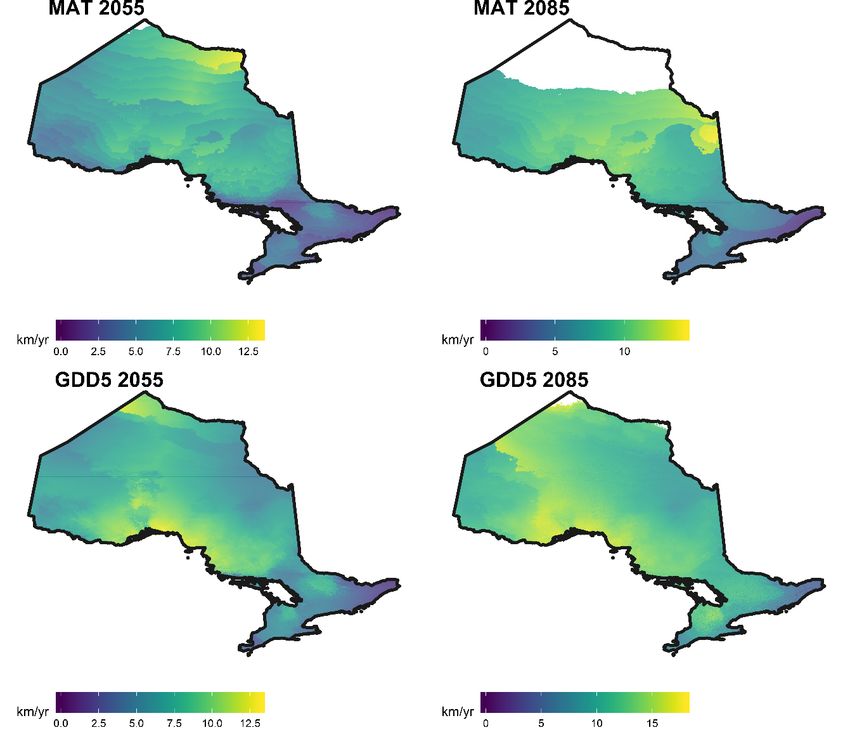
Spatially, VoCC of MAT and GDD5 increased from south to north, with the
northernmost and highest elevation areas of the province subjected to the fastest
climate velocities (Figure 3). For MAT (2085), no-analog climates were estimated in
much of the Far North. Southern Ontario, particularly the southeastern portion of the
province, was calculated to have the slowest climate velocities, perhaps resulting from
analog climates found in Michigan.
Climate Change Research Report CCRR-51 6Table 2. Summary of velocity of climate change (km·yr-1) for Ontario in mean annual temperature (MAT) and growing degree days >5 °C (GDD5) calculated from climate normals (1981–2010) and general circulation model ensemble mean climate projection (2055 and 2085) scenarios (RCP 4.5 and RCP 8.5). Variable-year- Min. First Median Mean Third Max. scenario quartile quartile MAT-2055-RCP 4.5 0 3.93 5.28 5.17 6.60 10.20 MAT-2085-RCP 4.5 0 3.77 4.91 4.69 5.76 9.48 MAT-2055-RCP 8.5 0 5.46 7.24 7.21 8.23 no-analog MAT-2085-RCP 8.5 0 7.56 9.59 28.09 11.73 no-analog GDD5-2055-RCP 4.5 0 4.88 5.97 6.20 7.37 13.60 GDD5-2085-RCP 4.5 0 4.28 5.15 5.26 6.14 9.85 GDD5-2055-RCP 8.5 0 6.04 7.27 7.36 8.63 13.13 GDD5-2085-RCP 8.5 0 10.62 11.83 12.94 13.43 no-analog Figure 2. Digital elevation model raster used to generate points for ClimateNA. The boundaries extend beyond Ontario to minimize no-analog climate conditions that may occur (i.e., represent regions that may have novel climate conditions), especially at northern margins where changes are happening fast. Climate Change Research Report CCRR-51 7
Figure 3. Velocity of climate change (km·yr-1) displayed as 1x1 km grid rasters for
mean annual temperature (MAT) and growing degree days >5 °C (GDD5) predicted in
2055 and 2085 under business as usual greenhouse gas emissions (RCP 8.5). White
areas indicate no-analog climate, i.e., novel, conditions.

Climate Change Research Report CCRR-51                                                8
4.0 Considering climate change in selecting protected
areas to support biodiversity conservation
    The selection and design of protected areas in Ontario are based on life science,
earth science, and cultural heritage criteria (OMNRF 2014). The life science criterion is
included to protect representative examples of the full range of biodiversity across the
province. The earth science criterion addresses the diversity of landforms, geologic
processes, and time periods, and the cultural heritage criterion is intended to protect
archaeological and historical features that represent landscape-related themes in
Ontario’s human history.

    For protected areas, climate change is most closely linked to the life science
criterion, and specifically the condition and ecological function aspects (OMNR 2014;
Figure 4). Condition is determined by assessing the level of human activities and the
least disturbed areas are selected for protection (Crins and Kor 2006). Since climate
change can disrupt ecological processes and threaten biodiversity (Walter et al. 2002),
other considerations for selecting sites to protect include promoting the persistence of
biodiversity (size, shape, connectivity, and hydrologic processes are important) where
ecological function is intact.

Figure 4. Selection and design criteria for protected areas in Ontario that are related to
climate change.

Climate Change Research Report CCRR-51                                                       9
5.0 Velocity of climate change applications
Here, we discuss how two metrics for VoCC, exposure and climate residence time,
can be used to 1) inform the selection and designation of new protected areas, 2) guide
planning in existing areas, and 3) identify potential habitats and refugia in protected
areas to support biodiversity conservation. The applications are discussed with specific
reference to Ontario but represent a sample of the global work completed using VoCC.
For a complete list of applications, see the review by Brito-Morales et al. (2018).
5.1 Exposure to climate change in relation to Ontario’s
ecological land classification hierarchy
Generally, populations or ecosystems occupying an area of relatively fast climate
velocity are more exposed to climate change than those subject to relatively slower
climate velocity. Thus, an estimate of climate change exposure is useful during initial
assessments of its potential threats to populations or ecosystems (Wiens et al. 2011,
Garcia et al. 2014, García Molinos et al. 2017). Greater exposure poses increased risk
to the cascade of ecological processes related to climate such as habitat availability,
phenology (timing of life history events such as flowering, leaf out, spawning
migrations), organismal growth and survival (Lynch et al. 2016), and ecological integrity
in protected areas.
Here, we summarize climate change exposure relative to different levels of Ontario’s
terrestrial ecological land classification (ELC) (Harold et al. 1998, Crins et al. 2009,
Akuma et al. 2015). The ELC classification levels are ecozones, ecoregions, and
ecodistricts. Ecozones are broadly defined based on continental climatic patterns and
major bedrock domains. Ecoregions are defined by sub-continental climatic regimes
and bedrock geology. Ecodistricts, which are the first spatial unit for protected area
selection in Ontario (Crins and Kor 2006), are characterized by distinctive patterns in
relief geology, geomorphology, vegetation, soils, water, and fauna. Illustrating the VoCC
for each of these ecological classification levels provides an assessment of the relative
exposure of different spatial scales to climate change.
The 1x1 km VoCC grids for MAT or GDD5, projected to 2055 or 2085 under RCP
4.5 or RCP 8.5, were summarized to describe VoCC for different ecological
classifications using the velox R package (Hunzinker 2017). Ecozones are shown by
MAT projected to 2055 under both GHG scenarios. Ecoregions are shown by MAT and
GDD5 under the business as usual GHG scenario (RCP 8.5) projected to 2055. Finally,
ecodistricts are shown by GDD5 under business as usual GHG emissions projected to
2085. While some examples of the results are presented below, data summaries for
Climate Change Research Report CCRR-51 10each ecological classification, time period, scenario, and climate variable are available
in the PAVoCC database (accessible via the authors, Aquatic Research and Monitoring
Section, MNRF).
Ecozones
Under the RCP 4.5 scenario projected to 2055, VoCC of MAT ranged from 0 to
about 10 km·yr-1 and was fastest in the Hudson Bay Lowlands Ecozone and slowest
throughout the Mixedwood Plains (Figure 5). This implies that populations or
ecosystems in the Far North are subject to faster rates of climate change than those in
southern Ontario. Under the RCP 8.5 business as usual GHG scenario, VoCC of MAT
ranged from 0 to 100 km·yr-1 from the climate normal period (1981–2010) to projected
climate in 2055. The maximum value (100 km·yr-1) represents no-analog climate
projected in the Hudson Bay Lowlands. Figures 3 and 6 illustrate the location of this no-
analog MAT climate region in the most northerly part the province.
Ecoregions
Under the RCP 8.5 scenario projected to 2055, MAT VoCC of Ontario’s ecoregions
ranged from 0 to about 7.5 km·yr-1. The MAT VoCCs increased with latitude, with the
slowest MAT VoCCs in the Lake Simcoe-Rideau Ecoregion. The fastest MAT VoCCs
were in the Northern Taiga and Hudson Bay Coast ecoregions. No-analog MAT values
were projected in the Far North (white area in Figure 6) meaning that no equivalent
climate exists in the area of interest (see Figure 3).
Under the business as usual GHG scenario and 2055 projection, GDD5 VoCC
ranged from 0 to about 13 km·yr-1 (figures 6 and 7). GDD5 VoCC was fasted for
ecoregions along the north shore of Lake Superior: Lake Nipigon, Lake Abitibi, and
Lake Temagami, with another pocket of fast GDD5 VoCCs in the Far North along the
Manitoba border. The Lake St. Joseph Ecoregion had moderate GDD5 VoCC with little
variation while the Lake Simcoe-Rideau Ecoregion had the slowest GDD5 VoCCs. The
Georgian Bay, Northern Taiga, and Lake Abitibi ecoregions had the widest ranges of
estimated GDD5 velocities (Figure 8).
Ecodistricts
Ecodistrict GDD5 velocities for RCP 8.5 predicted to 2085 ranged from 0 to about 17
km·yr-1 (figures 9 and 10). As expected, ecodistricts with the fastest velocities were in
the far northern areas of the province, with small pockets of no-analog climates along
Hudson Bay (Figure 9). Kemptville Ecodistrict had the slowest velocity in GDD5,
including several outliers at about 2 km·yr-1 (Figure 10). Northern ecodistricts such as
Schreiber, Kakabeka, Savanne and Tip Top Mountain were exposed to little variation
and relatively fast velocities in GDD5 (Figure 10).
Climate Change Research Report CCRR-51 11Figure 5. Velocity of climate change (km·yr-1) in mean annual temperature (MAT) for the climate normals period 1981 to 2010 and projected temperatures in 2055 under a greenhouse gas mitigation emissions scenario (RCP 4.5) and the ensemble mean general circulation model. Data are shown by ecozone (outlined in black). Climate Change Research Report CCRR-51 12
Figure 6. Velocity of climate change (km·yr-1) in mean annual temperature (MAT) for
the climate normals period 1981 to 2010 and projected temperatures in 2055 under a
business as usual greenhouse gas emissions scenario (RCP 8.5) and the ensemble
mean general circulation model. Data are shown by ecoregion (outlined in black).

Climate Change Research Report CCRR-51                                                13
Figure 7. Velocity of climate change (km·yr-1) in growing degree days >5 °C (GDD5) for
the climate normals period 1981 to 2010 and projected temperatures in 2055 under a
business as usual greenhouse gas emissions scenario (RCP 8.5) and the ensemble
mean general circulation model. Data are shown by ecoregion (outlined in black).

Climate Change Research Report CCRR-51                                              14
Figure 8. Box plot data, summarized by ecoregion, for velocity of climate change
(km·yr-1) in growing degree days >5 °C (GDD5) for the climate normals period 1981 to
2010 and predicted GDD5 in 2055 under a business as usual greenhouse gas
emissions scenario (RCP 8.5) and the ensemble mean general circulation model.

5.2 Exposure and selecting new protected areas
Quantifying climate change velocities and the corresponding exposure of ecosystems
and communities within and among land classification units is a step towards assessing
the relative vulnerability of Ontario’s ecosystems to climate change, including impacts to
biodiversity. Within the framework used to select new protected areas, exposure can be
one of the criteria used to assess condition, i.e., the level of human activities is
assessed to select sites with the least disturbance (Crins and Kor 2006). The summary
of magnitude and variation in VoCCs can be used to compare ecodistricts, and their
relative vulnerability to the impacts of climate change (Figure 10). Ecodistricts (and
areas/sites therein using velocities of 1x1 km grids) with relatively low and little variation
in exposure would be good candidates for protection because they are least likely to be
disturbed by climate change (figures 9 and 10). However, in Ontario, these ecodistricts
tend to include settled and disturbed landscapes where remaining natural systems are

Climate Change Research Report CCRR-51                                                     15
small and fragmented. The risk to ecological integrity from climate change in these
ecodistricts should be considered in context of local stresses and other changes in
climate (e.g., frequency of storm events).

Figure 9. Velocity of climate change (km·yr-1) in growing degree days >5 °C (GDD5) for
the climate normals period 1981 to 2010 and projected temperatures in 2085 under a
business as usual greenhouse gas emissions scenario (RCP 8.5) and the ensemble
mean general circulation model. Data are shown by ecodistrict; white areas in the Far
North (Dickey River and Wood Creek) indicate no-analog climates.

Climate Change Research Report CCRR-51                                                16
Figure 10. Box plot data, summarized by ecodistrict, for velocity of climate change (km·yr-1) in growing degree days >5 °C
(GDD5) for the climate normals period 1981 to 2010 and predicted GDD5 in 2055 under a business as usual greenhouse
gas emissions scenario (RCP 8.5) and the ensemble mean general circulation model. No-analog data are not shown.
Exposure is divided into low, moderate, and high based on quartile values of the velocity of climate change.

                                 Climate Change Research Report CCRR-51                                                17
The high exposure and high variation ecodistricts in northern Ontario occur in areas
with expansive tracks of intact natural ecosystems (figures 9 and 10). Selecting large
protected areas in these regions could help preserve those intact systems and increase
their resilience to climate change by increasing climate residency (see below). If it is not
feasible to establish large protected areas in high variation ecodistricts, areas/sites with
relatively low exposure or a network of relatively low exposure areas/sites could be
prioritized for protection.
5.3 Exposure and existing protected areas
Exposure can be used as a measure of climate change pressure in existing
protected areas and provides an estimate of the relative vulnerability of different regions
to change. For example, based on the ensemble GCM and RCP 8.5 emissions
scenario, MAT in Algonquin Provincial Park will change at speeds of 4.0 km·yr-1 to 7.7
km·yr-1 by 2085 (Figure 11). The park is on the Algonquin Dome, a regionally prominent
feature of Precambrian Canadian Shield reaching elevations of 587 metres above sea
level. Due to its elevation relative to the surrounding area, the Dome has a cool, wet
climate (Wester et al. 2018). In Algonquin Provincial Park, restrictions on forestry (land
cover change), limited fish species introductions, live bait prohibition, and regulations on
fish harvest have contributed to healthy, stable brook trout (Salvelinus fontinalis)
populations. Brook trout prefer cold water and increasing air temperatures and later ice-
out dates in Sproule Bay, Lake Opeongo since the 1960s (Ridgway et al. 2017) indicate
that warming air and water temperatures could put them at risk. The mean annual air
temperature velocities here suggest that exposure differs across the park and some
populations may be at greater risk than others (Figure 11).
Planning and management responses to varying exposures in existing parks will
depend on the defined objective(s). Continuing with brook trout in Algonquin Park as an
example, available planning or management options are to 1) prioritize areas where
VoCCs are relatively fast because they are the most likely to change or 2) prioritize
areas where VoCCs are relatively slow because they will be more likely to persist in a
changing climate. For brook trout inhabiting lakes exposed to rapid climate change,
management actions should aim to reduce stress on the populations or lakes. For
example, those lakes may be designated as sanctuaries or increased harvest
restrictions. Actions in slow velocity areas may include monitoring population status and
lake ecosystem health.
Climate change is compromising the effectiveness of some protected areas and
networks of protected areas as habitats and species ranges shift in response (Peters
and Darling 1985, Pressey et al. 2007, Game et al. 2011). Areas with slow VoCCs can
Climate Change Research Report CCRR-51 18be used to identify potential areas for stepping stones or corridors that allow species to
migrate and persist as the climate changes (D’Aloia et al. 2019). These stepping stones
or corridors may be temporarily or permanently integrated in existing protected area
networks and managed to maintain ecological function and support biodiversity.
Figure 11. Velocity of climate change in mean annual temperature (MAT; climate
normals from 1981 to 2010 relative to projected conditions in 2085 using an ensemble
mean general circulation model and RCP 8.5 emissions scenario) across Algonquin
Provincial Park and the surrounding landscape. For some of the identified lakes, brook
trout occupancy has not been recently verified. Red shading represents areas in the
park with the fastest climate velocities.
5.4 Exposure, refugia, and underrepresented habitats
If climate change modifies a species’ environment such that conditions become
unfavourable, the species’ range boundaries need to shift to achieve favourable
conditions (Thomas 2010, Chen et al. 2011, Poloczanska et al. 2013; except see Zhu et
al. 2012). Thus, organisms that cannot keep up with the pace of climate change (i.e.,
biotic velocity slower than climate velocity) may ultimately become extinct (Hiddink et al.
Climate Change Research Report CCRR-51 192015). Biotic velocities are estimates of species range shifts over time as species move
to stay in their climatic niche (Carroll et al. 2015). For example, birds have been shown
to track climate velocity where range shifts were multidirectional, depending on
interactions among climate variables (VanDerWal et al. 2013).
Refugia are habitats or environmental factors that offer spatiotemporal resistance or
resilience to biotic communities affected by human and natural disturbances (Sedell et
al. 1990). Climate refugia contain relatively slow-moving stable climates where
ecosystems may be expected to persist (Keppel et al. 2012, Harrison and Noss 2017).
In analyses of evolutionary history, contemporary patterns, and projected endemism,
VoCC has been used to characterize climate refugia across taxa (Sandel et al. 2011,
Abellán and Svenning 2014, Dalsgaard et al. 2014, Qiu et al. 2014, Roberts and
Hamann 2016). For example, Isaak et al. (2016) demonstrated that local climate
refuges exist for cold-water stream fishes in mountainous environments.
VoCC can also be useful when coupled with biologically relevant information (Reside
et al. 2014, Schueler et al. 2014, García Molinos et al. 2017, Stralberg et al. 2018).
Biotic velocity refugia represent areas of future climatic suitability that may be nearby
and accessible to a species’ current distribution (Ordonez and Williams 2013a,
Stralberg et al. 2018). As part of a North America-wide analysis using six metrics
(elevational diversity, heat load index diversity, current climatic diversity, ecotypic
diversity, land facet diversity, and backward climate velocity), Carroll et al. (2017)
ranked large areas of northern Ontario (Thunder Bay to Manitouwadge) as highly
important for conservation because of their capacity to act as climate refugia (Carroll et
al. 2017). Moreover, relative to the rest of North America, Ontario has been shown to
contain areas with both climate refugia and high species richness indices for song birds
and trees (Stralberg et al. 2018).
In Ontario, gap analyses are used to identify under or unrepresented
landform/vegetation features in undisturbed or least disturbed areas, and to set and
meet natural heritage targets (Crins and Kor 2006). Habitat types considered
inadequately represented in protected areas are given priority for conservation (OMNR
2014). Climate velocity can be incorporated into the gap analysis by evaluating how the
pace of climate change varies with underrepresented habitat types for a given
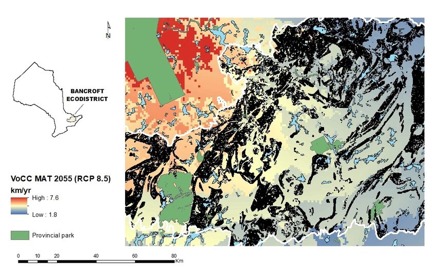
ecodistrict. For example, for the Bancroft Ecodistrict, climate velocity for mean annual
air temperature is slowest for underrepresented alvar and inland marsh and highest for
treed fen and sparse coniferous forest (figures 12 and 13). This suggests that the alvar
and inland marsh communities are less vulnerable to climate change and may be
refugia for alvar or marsh-dependent species. It also indicates that sparse coniferous
forests throughout the ecodistrict are most at risk and may require active management
for protection (Figure 13).
Climate Change Research Report CCRR-51 20To identify possible climate refugia for underrepresented habitat types, the database was sorted and the lowest five non-matching climate velocities for underrepresented habitat types were selected. This process identified possible climate refugia for open bog habitat west of Calabogie Lake (County of Renfrew), deciduous swamp and sparse deciduous forest habitats surrounding Moira Lake (County of Hastings), and bedrock habitat north of Stoco Lake (County of Renfrew; Figure 14). Spatially grouped habitats (e.g., near Moira Lake; Figure 14) in low velocity areas would have high conservation priority because they could provide climate refugia for many taxa. Species-specific assessments are needed to more comprehensively determine climate refugia for conserving biodiversity. Figure 12. Underrepresented habitat (black regions) in the Bancroft area in relation to provincial parks and climate velocity in mean annual temperature (MAT) predicted to 2055 under business as usual (RCP 8.5) greenhouse gas emissions. Bancroft Ecodistrict boundary is shown in white. Climate Change Research Report CCRR-51 21
Figure 13. Box plots of velocity of climate change (VoCC) of mean annual temperature
(MAT) predicted to 2055 under business as usual (RCP 8.5) greenhouse gas emissions
for underrepresented landform/vegetation types in the Bancroft Ecodistrict.

Figure 14. Underrepresented habitat types (vegetation type category) with the slowest
climate velocities (lowest five non-matching values for each type) in mean annual
temperature (predicted to 2055 under business as usual greenhouse gas emissions) in
the Bancroft Ecodistrict. Note the many underrepresented habitat types near Moira
Lake.

Climate Change Research Report CCRR-51                                             22
5.5 Climate residence times
    Climate residence is how long (typically measured in years) current climate will
persist in a protected area (Loarie et al. 2009). It can be computed from either the
original or distance-to-analog method as:

kma ÷ km·yr-1 = yr   [2]

where kma is the diameter of a circle of equivalent area to and centred on the area of
interest. It is divided by VoCC (km·yr-1) to obtain residency in years (Figure 15).

Figure 15. The calculation for climate residency time (years) in protected areas.
Velocity of climate change (VoCC) is given as a mean for the protected area. Surface
area (km2) is converted to a single dimension (km) from the diameter of a circle of equal
area to and centered on the protected area. Note that climate residence time depends
on the climate match threshold used to calculate VoCC.

    Residence times have been used in terrestrial and marine ecosystems to identify
how long it takes for an area/region to shift to unprecedented climates (Ackerly et al.
2010, Mora et al. 2013, Chen et al. 2016, Garciá Molinos et al. 2016) and to show that
some protected areas are insufficient to prevent future biodiversity loss (Chen et al.
2016). The relationship between climate residency and VoCC is typically inverse (i.e.,
residence time increases with protected area size or slower VoCC; Loarie et al. 2009),
but exceptions can occur based on the spatial configuration of the protected area. Very
large provincial parks such as Polar Bear and Wabakimi may have relatively long

Climate Change Research Report CCRR-51                                                   23
climate residence times despite their location in the north where climate velocities are
relatively fast (Figure 16). Additionally, small protected areas may have alarmingly short
climate residency times.
In Ontario under the GHG mitigation scenario projected to 2055, few protected areas
(Figure 16. (A) Climate residence times for Ontario protected areas under the 2055 general circulation model projection
(RCP 8.5) for mean annual temperature (climate match at ±0.25 °C). (B) Provincial parks with relatively high climate
residence times are shown relative to velocity of climate change in mean annual temperature (RCP 8.5).
Climate Change Research Report CCRR-51 25Figure 17. Frequency of provincial parks by climate residence time for growing degree
days >5 °C (GDD5) and mean annual temperature (MAT) predicted to 2055 under
mitigation (RCP 4.5) and business as usual (RCP 8.5) scenarios. In both cases, climate
matches are ±0.25 °C.
5.6 Climate residence times and existing protected areas
Management planning for protected areas in Ontario includes a temporal
component; often a 20-year time horizon or a 50-year time horizon for climate change
(OMNR 2014). Climate residence times can inform this aspect of planning and provide a
measure of time until the average climate conditions have changed given the specified
threshold (Figure 18). Climate residence time also gives a time frame for planning and
implementing management actions. Protected areas or parts of protected areas with
longer residence times may not require the same level of action as those with short
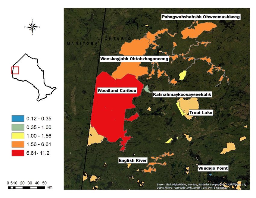
residence times (Figure 18). Based on a business as usual greenhouse gas emissions
scenario predicted in 2085, it would have taken about 11 years from 1996 (interim year
between 1981 and 2010) for the MAT in Woodland Caribou Provincial Park to increase
by 0.25°C. Under the same conditions, the much smaller Windigo Point Provincial Park
Climate Change Research Report CCRR-51 26would take only four months to change. Differences in climate residence time depend
on many factors (e.g., latitude, orientation, shape), with protected area size the most
influential. As mentioned above, the climate thresholds used to calculate residence time
will depend on the management planning objective and the sensitivity of the species or
communities of interest.
Figure 18. Climate residence times (yrs) for select protected areas in the northwest
near the Manitoba/Ontario border. Mean annual temperature (MAT) climate velocity was
predicted to 2085 under business as usual (RCP 8.5) greenhouse gas emissions.
Climate residence times depend on climate velocity and park size.
5.7 Climate residence times, habitat, and refugia
Climate residence times that are derived using the habitat preferences of species or
communities will provide measures of the theoretical length of time habitats will remain
suitable. For example, if it is known that a 5 °C increase in air temperature will affect the
growth and survival of a species of interest (for management planning), then residence
Climate Change Research Report CCRR-51 27time calculations can be used to rank protected areas based on how long they may
remain suitable for that species.
In general, protected areas with long residence times may act as refugia for many
species, and areas with complex topographies may offer microclimates (based on
exposure) that further buffer the effects of climate change (Loarie et al. 2009). Plans
that establish or improve connectivity among protected areas with long residence times
should bolster the resilience and effectiveness of protected area networks (Keeley et al.
2018). When protected areas are contiguous (e.g., Woodland Caribou and
Weeskayshak Ohtahzhoganeeng; Figure 18), climate residence time should be
calculated separately for each area because the management objectives, actions, and
plans may differ. However, the potential for species movement and refugia across
protected area boundaries should be considered. Where multiple, contiguous protected
areas may be managed as one unit and species movement is not restricted by barriers,
the whole area can be merged and used to calculate climate residence times.
6.0 Conclusions
The scientific community has reached a consensus on human-caused climate
change (Cook et al. 2013, 2016; Oreskes 2018; Ripple et al. 2019). The message to
policy makers has been clear: strengthen international co-operation and coordination to
better use resources, promote the free exchange of data, increase observational and
research capacity in developing nations, and communicate research advances in terms
that are relevant to decision making (IPCC 2001). Limit global warming to 1.5 °C or risk
serious losses of biodiversity, fisheries, and ecosystems; their function and services to
humans; and health, livelihoods, food security, water supply, human security, and
economic growth (IPCC 2018). As we move further into evolving and uncharted climate
conditions, protected areas are one of the strategies available to conserve biodiversity
and provide ecological representation (Table 3).
Ontario’s protected areas network has tremendous capacity to buffer climate change
risks and help achieve the recommendations set by the international community. Paired
with meaningful information about ecological communities and human-caused
disturbance, metrics such as climate change velocity can help us to estimate the effects
of climate change in existing and planned protected areas and inform broader
biodiversity conservation efforts in Ontario.
Climate Change Research Report CCRR-51 28Table 3. Summary of how velocity of climate change metrics, exposure, and residence
time can be incorporated into protected area management planning and biodiversity
conservation in Ontario.
Activity/goal Exposure: Residence time:
How fast (km·yr-1) is the How long (yr) is the current
climate changing? climate likely to persist?
Selecting new Prioritize large areas with slow NA
protected velocities for protection
areas
Managing Assume that condition and Use residence time to inform
existing ecological function will be more temporal targets in
protected intact in protected areas or management planning cycles
areas regions of protected areas with Prioritize protected areas with
slower velocities short residence times for
Prioritize areas with fast assessment and management
velocities for assessment and
intensive management
Use patchwork of slow velocity
areas to build stepping stones or
corridors for species habitat use
and migration
Understanding As potential for ecological Assume ecological function
habitat shifts function to change increases in likely to be compromised in
areas with fast velocities, assume protected areas with short
communities and species in residence times
those areas are more at risk from
climate change than communities
and species exposed to slow
velocities
Determining Depending on species habitat Assume protected areas with
refugia preferences, assume slow long residence times may
velocity areas may provide provide refugia
refugia
Climate Change Research Report CCRR-51 297.0 Literature cited
Abellán, P. and J.C. Svenning. 2014. Refugia within refugia — patterns in endemism
and genetic divergence are linked to Late Quaternary climate stability in the Iberian
Peninsula. Biological Journal of the Linnean Society 113: 13–28.
Ackerly, D.D., S.R. Loarie, W.K. Cornwell, S.B. Weiss, H. Hamilton, R. Branciforte and
N.J.B. Kraft. 2010. The geography of climate change: Implications for conservation
biogeography. Diversity and Distributions 16: 476–487.
Brito-Morales, I., J.G. Molinos, D.S. Schoeman, M.T. Burrows, E.S. Poloczanska, C.J.
Brown, S. Ferrier, T.D. Harwood, C.J. Klein, E. McDonald-Madden, P.J. Moore, J.M.
Pandolfi, J.E.M. Watson, A.S. Wenger and A.J. Richardson. 2018. Climate velocity
can inform conservation in a warming world. Trends in Ecology and Evolution 33:
441–457.
Carroll, C., D.R. Roberts, J.L. Michalak, J.J. Lawler, S.E. Nielsen, D. Stralberg, A.
Hamann, B.H. McRae and T. Wang. 2017. Scale-dependent complementarity of
climatic velocity and environmental diversity for identifying priority areas for
conservation under climate change. Global Change Biology 23: 4508–4520.
Chen, Y., J. Zhang, J. Jiang, S.E. Nielsen and F. He. 2016. Assessing the effectiveness
of China’s protected areas to conserve current and future amphibian diversity.
Diversity and Distributions 23: 146–157.
Cook, J., D. Nuccitelli, S.A. Green, M. Richardson, B. Winkler, R. Painting, R. Way, P.
Jacobs and A. Skuce. 2013. Quantifying the consensus on anthropogenic global
warming in the scientific literature. Environmental Research Letters 8: 024024.
Cook, J., N. Oreskes, P.T. Doran, W.R.L. Anderegg, B. Verheggen, EW. Maibach, J.S.
Carlton, S. Lewandowsky, A.G. Skuce and S.A. Green. 2016. Consensus on
consensus: A synthesis of consensus estimates on human-caused global warming.
Environmental Research Letters 11: 048002.
D’Aloia, C.C., I. Naujokaitis-Lewis, C. Blackford, C. Chu, J.M.R. Curtis, E. Darling, F.
Guichard, S.J. Leroux, A.C. Martensen, B. Rayfield, J.M. Sunday, A. Xuereb and M.
Fortin. 2019. Coupled networks of permanent protected areas and dynamic
conservation areas for biodiversity conservation under climate change. Frontiers in
Ecology and Evolution doi.org/10.3389/fevo.2019.00027
Dalsgaard, B., D.W. Carstensen, J. Fjeldså, P.K. Maruyama, C. Rahbek, B. Sandel, J.
Sonne, J. Svenning, Z. Wang and W.J. Sutherland. 2014. Determinants of bird
species richness, endemism, and island network roles in Wallacea and the West
Indies: Is geography sufficient or does current and historical climate matter? Ecology
and Evolution 4: 4019–4031.
Flato, G., N. Gillett, V. Arora, A. Cannon and J. Anstey. 2019. Modelling future climate
change. Pp. 74–111 in Bush, E. and D.S. Lemmen (eds.). Canada’s Changing
Climate Report. Government of Canada, Ottawa, ON.
Climate Change Research Report CCRR-51 30Vous pouvez aussi lire