PYQGIS DEVELOPER COOKBOOK - VERSION 2.2 QGIS PROJECT - QGIS DOCUMENTATION
←
→
Transcription du contenu de la page
Si votre navigateur ne rend pas la page correctement, lisez s'il vous plaît le contenu de la page ci-dessous
PyQGIS developer cookbook
                  Version 2.2

                QGIS Project

                  04 December 2014
Table des matières

1   Introduction                                                                                                                                                                                   1
    1.1 La Console Python . . . . . . . . . . . . . . . . . . . . . . . . . . . . . . . . . . . . . . . . . .                                                                                      1
    1.2 Extensions Python . . . . . . . . . . . . . . . . . . . . . . . . . . . . . . . . . . . . . . . . . .                                                                                      2
    1.3 Applications Python . . . . . . . . . . . . . . . . . . . . . . . . . . . . . . . . . . . . . . . . .                                                                                      2

2   Chargement de couches                                                                                                                                                                          5
    2.1 Couches vectorielles . . . . . . . . . . . . . . . . . . . . . . . . . . . . . . . . . . . . . . . . .                                                                                     5
    2.2 Couches raster . . . . . . . . . . . . . . . . . . . . . . . . . . . . . . . . . . . . . . . . . . . .                                                                                     6
    2.3 Map Layer Registry . . . . . . . . . . . . . . . . . . . . . . . . . . . . . . . . . . . . . . . . .                                                                                       7

3   Utiliser des couches raster                                                                                                                                                                     9
    3.1 Détails d’une couche .     .   .   .   .   .   .   .   .   .   .   .   .   .   .   .   .   .   .   .   .   .   .   .   .   .   .   .   .   .   .   .   .   .   .   .   .   .   .   .   .    9
    3.2 Drawing Style . . . .      .   .   .   .   .   .   .   .   .   .   .   .   .   .   .   .   .   .   .   .   .   .   .   .   .   .   .   .   .   .   .   .   .   .   .   .   .   .   .   .    9
    3.3 Rafraîchir les couches     .   .   .   .   .   .   .   .   .   .   .   .   .   .   .   .   .   .   .   .   .   .   .   .   .   .   .   .   .   .   .   .   .   .   .   .   .   .   .   .   11
    3.4 Query Values . . . . .     .   .   .   .   .   .   .   .   .   .   .   .   .   .   .   .   .   .   .   .   .   .   .   .   .   .   .   .   .   .   .   .   .   .   .   .   .   .   .   .   11

4   Utilisation de couches vectorielles                                                                                                                                                            13
    4.1 Iterating over Vector Layer . . . . . . . . . . . .                                .   .   .   .   .   .   .   .   .   .   .   .   .   .   .   .   .   .   .   .   .   .   .   .   .   .   13
    4.2 Modifying Vector Layers . . . . . . . . . . . . .                                  .   .   .   .   .   .   .   .   .   .   .   .   .   .   .   .   .   .   .   .   .   .   .   .   .   .   14
    4.3 Modifying Vector Layers with an Editing Buffer                                     .   .   .   .   .   .   .   .   .   .   .   .   .   .   .   .   .   .   .   .   .   .   .   .   .   .   15
    4.4 Using Spatial Index . . . . . . . . . . . . . . .                                  .   .   .   .   .   .   .   .   .   .   .   .   .   .   .   .   .   .   .   .   .   .   .   .   .   .   16
    4.5 Writing Vector Layers . . . . . . . . . . . . . .                                  .   .   .   .   .   .   .   .   .   .   .   .   .   .   .   .   .   .   .   .   .   .   .   .   .   .   17
    4.6 Memory Provider . . . . . . . . . . . . . . . . .                                  .   .   .   .   .   .   .   .   .   .   .   .   .   .   .   .   .   .   .   .   .   .   .   .   .   .   18
    4.7 Appearance (Symbology) of Vector Layers . . .                                      .   .   .   .   .   .   .   .   .   .   .   .   .   .   .   .   .   .   .   .   .   .   .   .   .   .   19

5   Manipulation de la géométrie                                                                                                                                                                   27
    5.1 Construction de géométrie . . . . . . . . . . . . . . . . . . . . . . . . . . . . . . . . . . . . . .                                                                                      27
    5.2 Accéder à la Géométrie . . . . . . . . . . . . . . . . . . . . . . . . . . . . . . . . . . . . . . .                                                                                       27
    5.3 Prédicats et opérations géométriques . . . . . . . . . . . . . . . . . . . . . . . . . . . . . . . .                                                                                       28

6   Support de projections                                                                                                                                                                         29
    6.1 Système de coordonnées de référence . . . . . . . . . . . . . . . . . . . . . . . . . . . . . . . .                                                                                        29
    6.2 Projections . . . . . . . . . . . . . . . . . . . . . . . . . . . . . . . . . . . . . . . . . . . . . .                                                                                    30

7   Utiliser le Canevas de carte                                                                                                                                                                   31
    7.1 Embedding Map Canvas . . . . . .                       .   .   .   .   .   .   .   .   .   .   .   .   .   .   .   .   .   .   .   .   .   .   .   .   .   .   .   .   .   .   .   .   .   31
    7.2 Using Map Tools with Canvas . . .                      .   .   .   .   .   .   .   .   .   .   .   .   .   .   .   .   .   .   .   .   .   .   .   .   .   .   .   .   .   .   .   .   .   32
    7.3 Rubber Bands and Vertex Markers .                      .   .   .   .   .   .   .   .   .   .   .   .   .   .   .   .   .   .   .   .   .   .   .   .   .   .   .   .   .   .   .   .   .   33
    7.4 Writing Custom Map Tools . . . .                       .   .   .   .   .   .   .   .   .   .   .   .   .   .   .   .   .   .   .   .   .   .   .   .   .   .   .   .   .   .   .   .   .   34
    7.5 Writing Custom Map Canvas Items                        .   .   .   .   .   .   .   .   .   .   .   .   .   .   .   .   .   .   .   .   .   .   .   .   .   .   .   .   .   .   .   .   .   35

8   Rendu cartographique et Impression                                                                                                                                                             37
    8.1 Simple Rendering . . . . . . . . . . . . . . . . . . . . . . . . . . . . . . . . . . . . . . . . . .                                                                                       37

                                                                                                                                                                                                    i
8.2 Output using Map Composer . . . . . . . . . . . . . . . . . . . . . . . . . . . . . . . . . . . . . 38
9 Expressions, Filtrage et Calcul de valeurs 41
9.1 Analyse syntaxique d’expressions . . . . . . . . . . . . . . . . . . . . . . . . . . . . . . . . . . 41
9.2 Évaluation des expressions . . . . . . . . . . . . . . . . . . . . . . . . . . . . . . . . . . . . . . 42
9.3 Exemples . . . . . . . . . . . . . . . . . . . . . . . . . . . . . . . . . . . . . . . . . . . . . . . 42
10 Lecture et sauvegarde de configurations 45
11 Communiquer avec l’utilisateur 47
11.1 Showing messages. The QgsMessageBar class. . . . . . . . . . . . . . . . . . . . . . . . . . . . 47
11.2 Afficher la progression . . . . . . . . . . . . . . . . . . . . . . . . . . . . . . . . . . . . . . . . 50
11.3 Journal . . . . . . . . . . . . . . . . . . . . . . . . . . . . . . . . . . . . . . . . . . . . . . . . 50
12 Développer des Extensions Python 53
12.1 Écriture d’une extension . . . . . . . . . . . . . . . . . . . . . . . . . . . . . . . . . . . . . . . 53
12.2 Contenu de l’extension . . . . . . . . . . . . . . . . . . . . . . . . . . . . . . . . . . . . . . . . 54
12.3 Documentation . . . . . . . . . . . . . . . . . . . . . . . . . . . . . . . . . . . . . . . . . . . . 58
13 IDE settings for writing and debugging plugins 59
13.1 A note on configuring your IDE on Windows . . . . . . . . . . . . . . . . . . . . . . . . . . . . 59
13.2 Débogage à l’aide d’Eclipse et PyDev . . . . . . . . . . . . . . . . . . . . . . . . . . . . . . . . 60
13.3 Débogage à l’aide de PDB . . . . . . . . . . . . . . . . . . . . . . . . . . . . . . . . . . . . . . 64
14 Using Plugin Layers 65
14.1 Subclassing QgsPluginLayer . . . . . . . . . . . . . . . . . . . . . . . . . . . . . . . . . . . . . 65
15 Compatibilité avec les versions précédentes de QGIS 67
15.1 Menu Extension . . . . . . . . . . . . . . . . . . . . . . . . . . . . . . . . . . . . . . . . . . . 67
16 Publier votre extension 69
16.1 Dépôt officiel des extensions Python . . . . . . . . . . . . . . . . . . . . . . . . . . . . . . . . . 69
17 Code Snippets 71
17.1 Comment appeler une méthode à l’aide d’un raccourci clavier . . . . . . . . . . . . . . . . . . . 71
17.2 How to toggle Layers (work around) . . . . . . . . . . . . . . . . . . . . . . . . . . . . . . . . 71
17.3 Comment accéder à la table attributaire des entités sélectionnées . . . . . . . . . . . . . . . . . . 72
18 Network analysis library 73
18.1 Information générale . . . . . . . . . . . . . . . . . . . . . . . . . . . . . . . . . . . . . . . . . 73
18.2 Building graph . . . . . . . . . . . . . . . . . . . . . . . . . . . . . . . . . . . . . . . . . . . . 73
18.3 Graph analysis . . . . . . . . . . . . . . . . . . . . . . . . . . . . . . . . . . . . . . . . . . . . 75
Index 81
iiCHAPITRE 1
Introduction
Ce document est à la fois un tutoriel et un guide de référence. Il ne liste pas tous les cas d’utilisation possibles,
mais donne une bonne idée générale des principales fonctionnalités.
Dès la version 0.9, QGIS intégrait un support optionnel pour le langage Python. Nous avons choisi Python car
c’est un des langages les plus adaptés pour la création de scripts. Les dépendances PyQGIS proviennent de SIP et
PyQt4. Le choix de l’utilisation de SIP plutôt que de SWIG plus généralement répandu est dû au fait que le noyau
de QGIS dépend des librairies Qt. Les dépendances Python pour Qt (PyQt) sont opérées via SIP, ce qui permet
une intégration parfaite de PyQGIS avec PyQt.
**A FAIRE : ** Faire fonctionner PyQGIS (compilation manuelle, débogage)
Il y a de nombreuses façons d’utiliser les dépendances python de QGIS ; elles sont mentionnées en détail dans les
sections suivantes :
– lancer des commandes dans la console Python de QGIS
– créer et utiliser des plugins en Python
– créer des applications personnalisées basées sur l’API QGIS
Il y a une documentation complète de l’API QGIS qui détaille les classes des librairies QGIS. l’API Python de
QGIS est presque identique à l’API en C++.
There are some resources about programming with PyQGIS on QGIS blog. See QGIS tutorial ported to Python for
some examples of simple 3rd party apps. A good resource when dealing with plugins is to download some plugins
from plugin repository and examine their code. Also, the python/plugins/ folder in your QGIS installation
contains some plugin that you can use to learn how to develop such plugin and how to perform some of the most
common tasks
1.1 La Console Python
Il est possible de tirer partie d’une console Python intégrée pour créer des scripts et les exécuter. La console
peut être ouverte grâce au menu : Plugins → Console Python. La console s’ouvre comme une fenêtre d’utilitaire
windows non modale :
La capture d’écran ci-dessus montre comment récupérer la couche sélectionnée dans la liste des couches, afficher
son identifiant et éventuellement, si c’est une couche vecteur, afficher le nombre d’entités. Pour interagir avec
l’environnement de QGIS, il y a une variable iface, instance de la classe QgsInterface. Cette interface
permet d’accéder au canevas de carte, aux menus, barres d’outils et autres composantes de l’application QGIS.
For convenience of the user, the following statements are executed when the console is started (in future it will be
possible to set further initial commands) :
from qgis.core import *
import qgis.utils
Pour ceux qui utilisent souvent la console, il peut être utile de définir un raccourci pour déclencher la console
(dans le menu Préférences → Configurer les raccourcis...)
1PyQGIS developer cookbook, Version 2.2
F IGURE 1.1 – La Console Python de QGIS
1.2 Extensions Python
QGIS permet d’enrichir ses fonctionnalités à l’aide d’extensions. Au départ, ce n’était possible qu’avec le langage
C++. Avec l’ajout du support de Python dans QGIS, il est également possible d’utiliser les extensions écrites
en Python. Le principal avantage sur des extensions C++ est leur simplicité de distribution (pas de compilation
nécessaire pour chaque plate-forme) et la facilité du développement.
De nombreuses extensions couvrant diverses fonctionnalités ont été écrites depuis l’introduction du
support de Python. L’installateur d’extensions permet aux utilisateurs de facilement chercher, met-
tre à niveau et supprimer les extensions Python. Voir la page du ‘ Dépôt des Extensions Python
‘_ pour diverses sources d’extensions.
Créer des extensions Python est simple. Voir Développer des Extensions Python pour des instructions détaillées.
1.3 Applications Python
Souvent lors du traitement de données SIG, il est très pratique de créer des scripts pour automatiser le processus au
lieu de faire la même tâche encore et encore. Avec PyQGIS, cela est parfaitement possible — importez le module
qgis.core, initialisez-le et vous êtes prêt pour le traitement.
Vous pouvez aussi souhaiter créer une application interactive utilisant certaines fonctionnalités SIG — mesurer des
données, exporter une carte en PDF ou toute autre fonction. Le module qgis.gui vous apporte différentes com-
posantes de l’interface, le plus notable étant le canevas de carte qui peut être facilement intégré dans l’application,
avec le support du zoom, du déplacement ou de tout autre outil personnalisé de cartographie.
1.3.1 Utiliser PyQGIS dans une application personnalisée
Note : ne pas utiliser qgis.py comme nom de script test — Python ne sera pas en mesure d’importer les
dépendances étant donné qu’elles sont occultées par le nom du script.
First of all you have to import qgis module, set QGIS path where to search for resources — database of projections,
providers etc. When you set prefix path with second argument set as True, QGIS will initialize all paths with
standard dir under the prefix directory. Calling initQgis() function is important to let QGIS search for the
available providers.
2 Chapitre 1. IntroductionPyQGIS developer cookbook, Version 2.2
from qgis.core import *
# supply path to where is your qgis installed
QgsApplication.setPrefixPath("/path/to/qgis/installation", True)
# load providers
QgsApplication.initQgis()
Maintenant, vous pouvez travailler avec l’API de QGIS — charger des couches et effectuer des traitements ou
lancer une interface graphique avec un canevas de carte. Les possibilités sont infinies :-)
Quand vous avez fini d’utiliser la librairie QGIS, appelez la fonction exitQgis() pour vous assurer que tout
est nettoyé (par ex, effacer le registre de couche cartographique et supprimer les couches) :
QgsApplication.exitQgis()
1.3.2 Exécuter des applications personnalisées
Vous devrez indiquer au système où trouver les librairies de QGIS et les modules Python appropriés s’ils ne sont
pas à un emplacement connu — autrement, Python se plaindra :
>>> import qgis.core
ImportError: No module named qgis.core
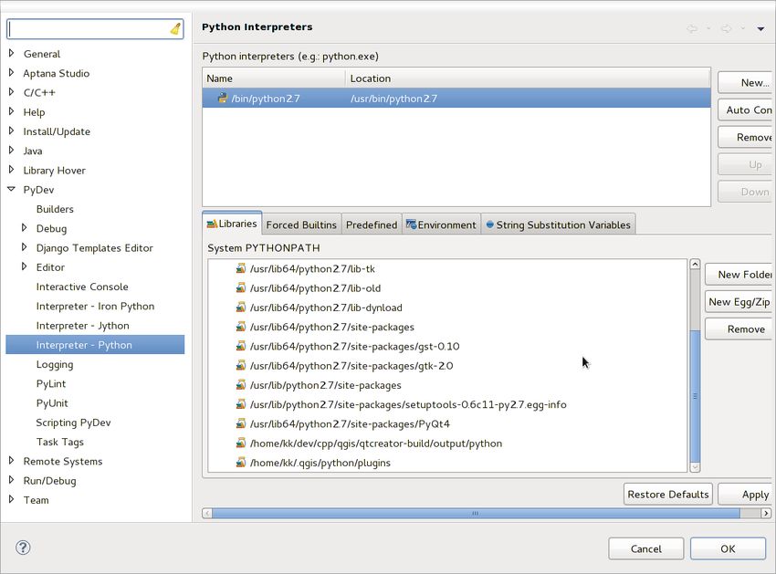
Ceci peut être corrigé en définissant la variable d’environnement PYTHONPATH. Dans les commandes suivantes,
qgispath doit être remplacé par le réel chemin d’accès au dossier d’installation de QGIS :
– sur Linux : export PYTHONPATH=/qgispath/share/qgis/python
– sur Windows : set PYTHONPATH=c :\qgispath\python
The path to the PyQGIS modules is now known, however they depend on qgis_core and qgis_gui libraries
(the Python modules serve only as wrappers). Path to these libraries is typically unknown for the operating system,
so you get an import error again (the message might vary depending on the system) :
>>> import qgis.core
ImportError: libqgis_core.so.1.5.0: cannot open shared object file: No such file or directory
Fix this by adding the directories where the QGIS libraries reside to search path of the dynamic linker :
– sur Linux : export LD_LIBRARY_PATH=/qgispath/lib
– sur Windows : set PATH=C :\qgispath ;%PATH%
These commands can be put into a bootstrap script that will take care of the startup. When deploying custom
applications using PyQGIS, there are usually two possibilities :
– require user to install QGIS on his platform prior to installing your application. The application installer should
look for default locations of QGIS libraries and allow user to set the path if not found. This approach has the
advantage of being simpler, however it requires user to do more steps.
– package QGIS together with your application. Releasing the application may be more challenging and the
package will be larger, but the user will be saved from the burden of downloading and installing additional
pieces of software.
The two deployment models can be mixed - deploy standalone application on Windows and Mac OS X, for Linux
leave the installation of QGIS up to user and his package manager.
1.3. Applications Python 3PyQGIS developer cookbook, Version 2.2 4 Chapitre 1. Introduction
CHAPITRE 2

                                                                        Chargement de couches

Ouvrons donc quelques couches de données. QGIS reconnaît les couches vectorielles et raster. En plus, des types
de couches personnalisés sont disponibles mais nous ne les aborderons pas ici.

2.1 Couches vectorielles

Pour charger une couche vectorielle, spécifiez l’identifiant de la source de données de la couche, un nom pour la
couche et le nom du fournisseur :
layer = QgsVectorLayer(data_source, layer_name, provider_name)
if not layer.isValid():
  print "Layer failed to load!"

L’identifiant de source de données est une chaîne de texte, spécifique à chaque type de fournisseur de données
vectorielles. Le nom de la couche est utilisée dans le widget liste de couches. Il est important de vérifier si la
couche a été chargée ou pas. Si ce n’était pas le cas, une instance de couche non valide est retournée.
La liste suivante montre comment accéder à différentes sources de données provenant de différents fournisseurs
de données vectorielles :
– La bibliothèque OGR (shapefiles et beaucoup d’autres formats) — la source de données est le chemin du fichier :
  vlayer = QgsVectorLayer("/path/to/shapefile/file.shp", \
    "layer_name_you_like", "ogr")

– PostGIS database — la source de donnée est une chaîne de texte contenant toutes les informations nécessaires à
  la création d’une connection à la base de données PostgreSQL. La classe QgsDataSourceURI peut générer
  ce texte pour vous. Notez que QGIS doit être compilé avec le support Postgres afin que ce fournisseur soit
  disponible. :
  uri = QgsDataSourceURI()
  # set host name, port, database name, username and password
  uri.setConnection("localhost", "5432", "dbname", "johny", "xxx")
  # set database schema, table name, geometry column and optionaly
  # subset (WHERE clause)
  uri.setDataSource("public", "roads", "the_geom", "cityid = 2643")

  vlayer = QgsVectorLayer(uri.uri(), "layer_name_you_like", "postgres")

– CSV ou autres fichiers de texte délimité — pour ouvrir un fichier délimité par le point-virgule, ayant des champs
  “x” et “y” respectivement pour coordonnées x et y, vous devriez utiliser quelque chose comme ceci :
  uri = "/some/path/file.csv?delimiter=%s&xField=%s&yField=%s" % (";", "x", "y")
  vlayer = QgsVectorLayer(uri, "layer_name_you_like", "delimitedtext")

                                                                                                                 5
PyQGIS developer cookbook, Version 2.2
Note : from QGIS version 1.7 the provider string is structured as a URL, so the path must be prefixed with
file ://. Also it allows WKT (well known text) formatted geomtries as an alternative to “x” and “y” fields, and
allows the coordinate reference system to be specified. For example
uri = "file:///some/path/file.csv?delimiter=%s&crs=epsg:4723&wktField=%s" \
% (";", "shape")
– GPX files — the “gpx” data provider reads tracks, routes and waypoints from gpx files. To open a file, the type
(track/route/waypoint) needs to be specified as part of the url
uri = "path/to/gpx/file.gpx?type=track"
vlayer = QgsVectorLayer(uri, "layer_name_you_like", "gpx")
– Base de données Spatialite — supporté depuis la version 1.1 de QGIS. Tout comme avec les bases de données
PostGIS, la classe QgsDataSourceURI peut être utilisée pour générer l’identifiant de la source de données :
uri = QgsDataSourceURI()
uri.setDatabase(’/home/martin/test-2.3.sqlite’)
schema = ’’
table = ’Towns’
geom_column = ’Geometry’
uri.setDataSource(schema, table, geom_colum)
display_name = ’Towns’
vlayer = QgsVectorLayer(uri.uri(), display_name, ’spatialite’)
– MySQL WKB-based geometries, through OGR — data source is the connection string to the table
uri = "MySQL:dbname,host=localhost,port=3306,user=root,password=xxx|\
layername=my_table"
vlayer = QgsVectorLayer( uri, "my_table", "ogr" )
– WFS connection :. the connection is defined with a URI and using the WFS provider
uri = "http://localhost:8080/geoserver/wfs?srsname=EPSG:23030&typename=\
union&version=1.0.0&request=GetFeature&service=WFS",
vlayer = QgsVectorLayer("my_wfs_layer", "WFS")
The uri can be created using the standard urllib library.
params = {
’service’: ’WFS’,
’version’: ’1.0.0’,
’request’: ’GetFeature’,
’typename’: ’union’,
’srsname’: "EPSG:23030"
}
uri = ’http://localhost:8080/geoserver/wfs?’ + \
urllib.unquote(urllib.urlencode(params))
And you can also use the
2.2 Couches raster
For accessing raster files, GDAL library is used. It supports a wide range of file formats. In case you have troubles
with opening some files, check whether your GDAL has support for the particular format (not all formats are
available by default). To load a raster from a file, specify its file name and base name
6 Chapitre 2. Chargement de couchesPyQGIS developer cookbook, Version 2.2 fileName = "/path/to/raster/file.tif" fileInfo = QFileInfo(fileName) baseName = fileInfo.baseName() rlayer = QgsRasterLayer(fileName, baseName) if not rlayer.isValid(): print "Layer failed to load!" Les couches raster peuvent également être créées à partir d’un service WCS. layer_name = ’elevation’ uri = QgsDataSourceURI() uri.setParam (’url’, ’http://localhost:8080/geoserver/wcs’) uri.setParam ( "identifier", layer_name) rlayer = QgsRasterLayer(uri, ’my_wcs_layer’, ’wcs’) Alternatively you can load a raster layer from WMS server. However currently it’s not possible to access GetCa- pabilities response from API — you have to know what layers you want urlWithParams = ’url=http://wms.jpl.nasa.gov/wms.cgi&layers=global_mosaic&\ styles=pseudo&format=image/jpeg&crs=EPSG:4326’ rlayer = QgsRasterLayer(urlWithParams, ’some layer name’, ’wms’) if not rlayer.isValid(): print "Layer failed to load!" 2.3 Map Layer Registry If you would like to use the opened layers for rendering, do not forget to add them to map layer registry. The map layer registry takes ownership of layers and they can be later accessed from any part of the application by their unique ID. When the layer is removed from map layer registry, it gets deleted, too. Adding a layer to the registry : QgsMapLayerRegistry.instance().addMapLayer(layer) Les couches sont automatiquement supprimées lorsque vous quittez, mais si vous souhaitez explicitement sup- primer la couche, utilisez : QgsMapLayerRegistry.instance().removeMapLayer(layer_id) A FAIRE : More about map layer registry ? 2.3. Map Layer Registry 7
PyQGIS developer cookbook, Version 2.2

8                                        Chapitre 2. Chargement de couches
CHAPITRE 3

                                                                      Utiliser des couches raster

Cette section liste différentes opérations réalisables avec des couches raster.

3.1 Détails d’une couche

A raster layer consists of one or more raster bands - it is referred to as either single band or multi band raster. One
band represents a matrix of values. Usual color image (e.g. aerial photo) is a raster consisting of red, blue and
green band. Single band layers typically represent either continuous variables (e.g. elevation) or discrete variables
(e.g. land use). In some cases, a raster layer comes with a palette and raster values refer to colors stored in the
palette.
>>> rlayer.width(), rlayer.height()
(812, 301)
>>> rlayer.extent()
u’12.095833,48.552777 : 18.863888,51.056944’
>>> rlayer.rasterType()
2 # 0 = GrayOrUndefined (single band), 1 = Palette (single band), 2 = Multiband
>>> rlayer.bandCount()
3
>>> rlayer.metadata()
u’Driver:...’
>>> rlayer.hasPyramids()
False

3.2 Drawing Style

When a raster layer is loaded, it gets a default drawing style based on its type. It can be altered either in raster
layer properties or programmatically. The following drawing styles exist :
 In-      Constante :                      Commentaire
 dex      QgsRasterLater.X
 1        SingleBandGray                   Single band image drawn as a range of gray colors
 2        SingleBandPseudoColor            Single band image drawn using a pseudocolor algorithm
 3        PalettedColor                    “Palette” image drawn using color table
 4        PalettedSingleBandGray           “Palette” layer drawn in gray scale
 5        PalettedSingleBandPseudo-        “Palette” layerdrawn using a pseudocolor algorithm
          Color
 7        MultiBandSingleBandGray          Layer containing 2 or more bands, but a single band drawn as a range
                                           of gray colors
 8        MultiBandSingle-                 Layer containing 2 or more bands, but a single band drawn using a
          BandPseudoColor                  pseudocolor algorithm
 9        MultiBandColor                   Layer containing 2 or more bands, mapped to RGB color space.

                                                                                                                     9
PyQGIS developer cookbook, Version 2.2
To query the current drawing style :
>>> rlayer.drawingStyle()
9
Single band raster layers can be drawn either in gray colors (low values = black, high values = white) or with a
pseudocolor algorithm that assigns colors for values from the single band. Single band rasters with a palette can be
additionally drawn using their palette. Multiband layers are typically drawn by mapping the bands to RGB colors.
Other possibility is to use just one band for gray or pseudocolor drawing.
The following sections explain how to query and modify the layer drawing style. After doing the changes, you
might want to force update of map canvas, see Rafraîchir les couches.
TODO : contrast enhancements, transparency (no data), user defined min/max, band statistics
3.2.1 Single Band Rasters
They are rendered in gray colors by default. To change the drawing style to pseudocolor :
>>> rlayer.setDrawingStyle(QgsRasterLayer.SingleBandPseudoColor)
>>> rlayer.setColorShadingAlgorithm(QgsRasterLayer.PseudoColorShader)
The PseudoColorShader is a basic shader that highlighs low values in blue and high values in red. Another,
FreakOutShader uses more fancy colors and according to the documentation, it will frighten your granny and
make your dogs howl.
There is also ColorRampShader which maps the colors as specified by its color map. It has three modes of
interpolation of values :
– linear (INTERPOLATED) : resulting color is linearly interpolated from the color map entries above and below
the actual pixel value
– discrete (DISCRETE) : color is used from the color map entry with equal or higher value
– exact (EXACT) : color is not interpolated, only the pixels with value equal to color map entries are drawn
To set an interpolated color ramp shader ranging from green to yellow color (for pixel values from 0 to 255) :
>>> rlayer.setColorShadingAlgorithm(QgsRasterLayer.ColorRampShader)
>>> lst = [ QgsColorRampShader.ColorRampItem(0, QColor(0,255,0)), \
QgsColorRampShader.ColorRampItem(255, QColor(255,255,0)) ]
>>> fcn = rlayer.rasterShader().rasterShaderFunction()
>>> fcn.setColorRampType(QgsColorRampShader.INTERPOLATED)
>>> fcn.setColorRampItemList(lst)
Pour retourner aux niveaux de gris par défaut, utilisez :
>>> rlayer.setDrawingStyle(QgsRasterLayer.SingleBandGray)
3.2.2 Multi Band Rasters
By default, QGIS maps the first three bands to red, green and blue values to create a color image (this is the
MultiBandColor drawing style. In some cases you might want to override these setting. The following code
interchanges red band (1) and green band (2) :
>>> rlayer.setGreenBandName(rlayer.bandName(1))
>>> rlayer.setRedBandName(rlayer.bandName(2))
In case only one band is necessary for visualization of the raster, single band drawing can be chosen — either gray
levels or pseudocolor, see previous section :
>>> rlayer.setDrawingStyle(QgsRasterLayer.MultiBandSingleBandPseudoColor)
>>> rlayer.setGrayBandName(rlayer.bandName(1))
>>> rlayer.setColorShadingAlgorithm(QgsRasterLayer.PseudoColorShader)
>>> # now set the shader
10 Chapitre 3. Utiliser des couches rasterPyQGIS developer cookbook, Version 2.2
3.3 Rafraîchir les couches
Si vous avez effectué des modifications sur le style d’une couche et tenez à ce qu’elles soient automatiquement
visibles pour l’utilisateur, appelez ces méthodes :
if hasattr(layer, "setCacheImage"): layer.setCacheImage(None)
layer.triggerRepaint()
The first call will ensure that the cached image of rendered layer is erased in case render caching is turned on. This
functionality is available from QGIS 1.4, in previous versions this function does not exist — to make sure that the
code works with all versions of QGIS, we first check whether the method exists.
La deuxième commande émet un signal forçant l’actualisation de tout canevas de carte contenant la couche.
With WMS raster layers, these commands do not work. In this case, you have to do it explicitily :
layer.dataProvider().reloadData()
layer.triggerRepaint()
In case you have changed layer symbology (see sections about raster and vector layers on how to do that), you
might want to force QGIS to update the layer symbology in the layer list (legend) widget. This can be done as
follows (iface is an instance of QgisInterface) :
iface.legendInterface().refreshLayerSymbology(layer)
3.4 Query Values
To do a query on value of bands of raster layer at some specified point :
ident = rlayer.dataProvider().identify(QgsPoint(15.30,40.98), \
QgsRaster.IdentifyFormatValue)
if ident.isValid():
print ident.results()
The results method in this case returs a dictionary, with band indices as keys, and band values as values.
{1: 17, 2: 220}
3.3. Rafraîchir les couches 11PyQGIS developer cookbook, Version 2.2 12 Chapitre 3. Utiliser des couches raster
CHAPITRE 4

                                                       Utilisation de couches vectorielles

Cette section résume les diverses actions possibles sur les couches vectorielles.

4.1 Iterating over Vector Layer

Iterating over the features in a vector layer is one of the most common tasks. Below is an example of the simple
basic code to perform this task and showing some information about each feature. the layer variable is assumed
to have a QgsVectorLayer object
iter = layer.getFeatures()
for feature in iter:
  # retreive every feature with its geometry and attributes
    # fetch geometry
    geom = feature.geometry()
    print "Feature ID %d: " % feature.id()

     # show some information about the feature
     if geom.type() == QGis.Point:
       x = geom.asPoint()
       print "Point: " + str(x)
     elif geom.type() == QGis.Line:
       x = geom.asPolyline()
       print "Line: %d points" % len(x)
     elif geom.type() == QGis.Polygon:
       x = geom.asPolygon()
       numPts = 0
       for ring in x:
         numPts += len(ring)
       print "Polygon: %d rings with %d points" % (len(x), numPts)
     else:
       print "Unknown"

     # fetch attributes
     attrs = feature.attributes()

     # attrs is a list. It contains all the attribute values of this feature
     print attrs

Attributes can be refered by index.
idx = layer.fieldNameIndex(’name’)
print feature.attributes()[idx]

                                                                                                             13
PyQGIS developer cookbook, Version 2.2
4.1.1 Iterating over selected features
4.1.2 Convenience methods
For the above cases, and in case you need to consider selection in a vector layer in case it exist, you can use the
features() method from the buil-in processing plugin, as follows :
import processing
features = processing.features(layer)
for feature in features:
#Do whatever you need with the feature
This will iterate over all the features in the layer, in case there is no selection, or over the selected features
otherwise.
if you only need selected features, you can use the :func : selectedFeatures method from vector layer :
selection = layer.selectedFeatures()
print len(selection)
for feature in selection:
#Do whatever you need with the feature
4.1.3 Iterating over a subset of features
If you want to iterate over a given subset of features in a layer, such as those within a given area, you have to add
a QgsFeatureRequest object to the getFeatures() call. Here’s an example
request=QgsFeatureRequest()
request.setFilterRect(areaOfInterest)
for f in layer.getFeatures(request):
...
The request can be used to define the data retrieved for each feature, so the iterator returns all features, but return
partial data for each of them.
request.setSubsetOfFields([0,2]) # Only return selected fields
request.setSubsetOfFields([’name’,’id’],layer.fields()) # More user friendly version
request.setFlags( QgsFeatureRequest.NoGeometry ) # Don’t return geometry objects
4.2 Modifying Vector Layers
Most vector data providers support editing of layer data. Sometimes they support just a subset of possible editing
actions. Use the capabilities() function to find out what set of functionality is supported :
caps = layer.dataProvider().capabilities()
By using any of following methods for vector layer editing, the changes are directly committed to the underlying
data store (a file, database etc). In case you would like to do only temporary changes, skip to the next section that
explains how to do modifications with editing buffer.
4.2.1 Ajout d’Entités
Create some QgsFeature instances and pass a list of them to provider’s addFeatures() method. It will
return two values : result (true/false) and list of added features (their ID is set by the data store) :
14 Chapitre 4. Utilisation de couches vectoriellesPyQGIS developer cookbook, Version 2.2
if caps & QgsVectorDataProvider.AddFeatures:
feat = QgsFeature()
feat.addAttribute(0,"hello")
feat.setGeometry(QgsGeometry.fromPoint(QgsPoint(123,456)))
(res, outFeats) = layer.dataProvider().addFeatures( [ feat ] )
4.2.2 Suppression d’Entités
To delete some features, just provide a list of their feature IDs :
if caps & QgsVectorDataProvider.DeleteFeatures:
res = layer.dataProvider().deleteFeatures([ 5, 10 ])
4.2.3 Modifier des Entités
It is possible to either change feature’s geometry or to change some attributes. The following example first changes
values of attributes with index 0 and 1, then it changes the feature’s geometry :
fid = 100 # ID of the feature we will modify
if caps & QgsVectorDataProvider.ChangeAttributeValues:
attrs = { 0 : "hello", 1 : 123 }
layer.dataProvider().changeAttributeValues({ fid : attrs })
if caps & QgsVectorDataProvider.ChangeGeometries:
geom = QgsGeometry.fromPoint(QgsPoint(111,222))
layer.dataProvider().changeGeometryValues({ fid : geom })
4.2.4 Ajout et Suppression de Champs
To add fields (attributes), you need to specify a list of field defnitions. For deletion of fields just provide a list of
field indexes.
if caps & QgsVectorDataProvider.AddAttributes:
res = layer.dataProvider().addAttributes( [ QgsField("mytext", \
QVariant.String), QgsField("myint", QVariant.Int) ] )
if caps & QgsVectorDataProvider.DeleteAttributes:
res = layer.dataProvider().deleteAttributes( [ 0 ] )
After adding or removing fields in the data provider the layer’s fields need to be updated because the changes are
not automatically propagated.
layer.updateFields()
4.3 Modifying Vector Layers with an Editing Buffer
When editing vectors within QGIS application, you have to first start editing mode for a particular layer, then do
some modifications and finally commit (or rollback) the changes. All the changes you do are not written until
you commit them — they stay in layer’s in-memory editing buffer. It is possible to use this functionality also
programmatically — it is just another method for vector layer editing that complements the direct usage of data
providers. Use this option when providing some GUI tools for vector layer editing, since this will allow user to
decide whether to commit/rollback and allows the usage of undo/redo. When committing changes, all changes
from the editing buffer are saved to data provider.
4.3. Modifying Vector Layers with an Editing Buffer 15PyQGIS developer cookbook, Version 2.2
To find out whether a layer is in editing mode, use isEditing() — the editing functions work only when the
editing mode is turned on. Usage of editing functions :
# add two features (QgsFeature instances)
layer.addFeatures([feat1,feat2])
# delete a feature with specified ID
layer.deleteFeature(fid)
# set new geometry (QgsGeometry instance) for a feature
layer.changeGeometry(fid, geometry)
# update an attribute with given field index (int) to given value (QVariant)
layer.changeAttributeValue(fid, fieldIndex, value)
# add new field
layer.addAttribute(QgsField("mytext", QVariant.String))
# remove a field
layer.deleteAttribute(fieldIndex)
In order to make undo/redo work properly, the above mentioned calls have to be wrapped into undo commands.
(If you do not care about undo/redo and want to have the changes stored immediately, then you will have easier
work by editing with data provider.) How to use the undo functionality
layer.beginEditCommand("Feature triangulation")
# ... call layer’s editing methods ...
if problem_occurred:
layer.destroyEditCommand()
return
# ... more editing ...
layer.endEditCommand()
The beginEndCommand() will create an internal “active” command and will record subsequent changes
in vector layer. With the call to endEditCommand() the command is pushed onto the undo stack and the
user will be able to undo/redo it from GUI. In case something went wrong while doing the changes, the
destroyEditCommand() method will remove the command and rollback all changes done while this com-
mand was active.
To start editing mode, there is startEditing() method, to stop editing there are commitChanges() and
rollback() — however normally you should not need these methods and leave this functionality to be triggered
by the user.
4.4 Using Spatial Index
Spatial indexes can dramatically improve the performance of your code if you need to do frequent queries to a
vector layer. Imagin, for instance, that you are writing an interpolation algorithm, and that for a given location you
need to know the 10 closest point from a points layer„ in order to use those point for calculating the interpolated
value. Without a spatial index, the only way for QGIS to find those 10 points is to compute the distance from each
and every point to the specified location and then compare those distances. This can be a very time consuming
task, specilly if it needs to be repeated fro several locations. If a spatial index exists for the layer, the operation is
much more effective.
Think of a layer withou a spatial index as a telephone book in which telephone number are not orderer or indexed.
The only way to find the telephone number of a given person is to read from the beginning until you find it.
Spatial indexes are not created by default for a QGIS vector layer, but you can create them easily. This is what you
have to do.
1. create spatial index — the following code creates an empty index :
16 Chapitre 4. Utilisation de couches vectoriellesPyQGIS developer cookbook, Version 2.2
index = QgsSpatialIndex()
2. add features to index — index takes QgsFeature object and adds it to the internal data structure. You can
create the object manually or use one from previous call to provider’s nextFeature()
index.insertFeature(feat)
3. once spatial index is filled with some values, you can do some queries :
# returns array of feature IDs of five nearest features
nearest = index.nearestNeighbor(QgsPoint(25.4, 12.7), 5)
# returns array of IDs of features which intersect the rectangle
intersect = index.intersects(QgsRectangle(22.5, 15.3, 23.1, 17.2))
4.5 Writing Vector Layers
You can write vector layer files using QgsVectorFileWriter class. It supports any other kind of vector file
that OGR supports (shapefiles, GeoJSON, KML and others).
Il y a deux façons d’exporter une couche vectorielle :
– from an instance of QgsVectorLayer :
error = QgsVectorFileWriter.writeAsVectorFormat(layer, "my_shapes.shp", \
"CP1250", None, "ESRI Shapefile")
if error == QgsVectorFileWriter.NoError:
print "success!"
error = QgsVectorFileWriter.writeAsVectorFormat(layer, "my_json.json", \
"utf-8", None, "GeoJSON")
if error == QgsVectorFileWriter.NoError:
print "success again!"
The third parameter specifies output text encoding. Only some drivers need this for correct operation - shapefiles
are one of those — however in case you are not using international characters you do not have to care much
about the encoding. The fourth parameter that we left as None may specify destination CRS — if a valid
instance of QgsCoordinateReferenceSystem is passed, the layer is transformed to that CRS.
For valid driver names please consult the supported formats by OGR — you should pass the value in ‘the
“Code” column as the driver name. Optionally you can set whether to export only selected features, pass further
driver-specific options for creation or tell the writer not to create attributes — look into the documentation for
full syntax.
– directly from features :
# define fields for feature attributes. A list of QgsField objects is needed
fields = [QgsField("first", QVariant.Int),
QgsField("second", QVariant.String) ]
# create an instance of vector file writer, which will create the vector file.
# Arguments:
# 1. path to new file (will fail if exists already)
# 2. encoding of the attributes
# 3. field map
# 4. geometry type - from WKBTYPE enum
# 5. layer’s spatial reference (instance of
# QgsCoordinateReferenceSystem) - optional
# 6. driver name for the output file
writer = QgsVectorFileWriter("my_shapes.shp", "CP1250", fields, \
QGis.WKBPoint, None, "ESRI Shapefile")
if writer.hasError() != QgsVectorFileWriter.NoError:
4.5. Writing Vector Layers 17PyQGIS developer cookbook, Version 2.2
print "Error when creating shapefile: ", writer.hasError()
# add a feature
fet = QgsFeature()
fet.setGeometry(QgsGeometry.fromPoint(QgsPoint(10,10)))
fet.setAttributes([1, "text"])
writer.addFeature(fet)
# delete the writer to flush features to disk (optional)
del writer
4.6 Memory Provider
Memory provider is intended to be used mainly by plugin or 3rd party app developers. It does not store data on
disk, allowing developers to use it as a fast backend for some temporary layers.
The provider supports string, int and double fields.
The memory provider also supports spatial indexing, which is enabled by calling the provider’s
createSpatialIndex() function. Once the spatial index is created you will be able to iterate over features
within smaller regions faster (since it’s not necessary to traverse all the features, only those in specified rectangle).
A memory provider is created by passing "memory" as the provider string to the QgsVectorLayer construc-
tor.
The constructor also takes a URI defining the geometry type of the layer, one of : "Point", "LineString",
"Polygon", "MultiPoint", "MultiLineString", or "MultiPolygon".
The URI can also specify the coordinate reference system, fields, and indexing of the memory provider in the URI.
The syntax is :
crs=definition Spécifie le système de coordonnée de référence, où définition peut être sous n’importe laquelle
des formes acceptées par QgsCoordinateReferenceSystem.createFromString()
index=yes Spécifie que le fournisseur utilisera un index spatial
field=name :type(length,precision) Specifies an attribute of the layer. The attribute has a name, and optionally a
type (integer, double, or string), length, and precision. There may be multiple field definitions.
The following example of a URI incorporates all these options :
"Point?crs=epsg:4326&field=id:integer&field=name:string(20)&index=yes"
The following example code illustrates creating and populating a memory provider :
# create layer
vl = QgsVectorLayer("Point", "temporary_points", "memory")
pr = vl.dataProvider()
# add fields
pr.addAttributes( [ QgsField("name", QVariant.String),
QgsField("age", QVariant.Int),
QgsField("size", QVariant.Double) ] )
# add a feature
fet = QgsFeature()
fet.setGeometry( QgsGeometry.fromPoint(QgsPoint(10,10)) )
fet.setAttributes(["Johny", 2, 0.3])
pr.addFeatures([fet])
# update layer’s extent when new features have been added
# because change of extent in provider is not propagated to the layer
vl.updateExtents()
18 Chapitre 4. Utilisation de couches vectoriellesPyQGIS developer cookbook, Version 2.2
Finally, let’s check whether everything went well :
# show some stats
print "fields:", len(pr.fields())
print "features:", pr.featureCount()
e = layer.extent()
print "extent:", e.xMin(),e.yMin(),e.xMax(),e.yMax()
# iterate over features
f = QgsFeature()
features = vl.getFeatures()
for f in features:
print "F:",f.id(), f.attributes(), f.geometry().asPoint()
4.7 Appearance (Symbology) of Vector Layers
When a vector layer is being rendered, the appearance of the data is given by renderer and symbols associated
with the layer. Symbols are classes which take care of drawing of visual representation of features, while renderers
determine what symbol will be used for a particular feature.
The renderer for a given layer can obtained as shown below :
renderer = layer.rendererV2()
And with that reference, let us explore it a bit :
print "Type:", rendererV2.type()
There are several known renderer types available in QGIS core library :
Type Class Description
singleSymbol QgsSingleSymbolRendererV2 Renders all features with the same symbol
catego- Renders features using a different symbol for each
QgsCategorizedSymbolRendererV2
rizedSymbol category
graduatedSym- Renders features using a different symbol for each
QgsGraduatedSymbolRendererV2
bol range of values
There might be also some custom renderer types, so never make an assumption there are just these types. You can
query QgsRendererV2Registry singleton to find out currently available renderers.
It is possible to obtain a dump of a renderer contents in text form — can be useful for debugging :
print rendererV2.dump()
You can get the symbol used for rendering by calling symbol() method and change it with setSymbol()
method (note for C++ devs : the renderer takes ownership of the symbol.)
You can query and set attribute name which is used for classification : use classAttribute() and
setClassAttribute() methods.
To get a list of categories :
for cat in rendererV2.categories():
print "%s: %s :: %s" % (cat.value().toString(), cat.label(), str(cat.symbol()))
Where value() is the value used for discrimination between categories, label() is a text used for category
description and symbol() method returns assigned symbol.
The renderer usually stores also original symbol and color ramp which were used for the classification :
sourceColorRamp() and sourceSymbol() methods.
This renderer is very similar to the categorized symbol renderer described above, but instead of one attribute value
per class it works with ranges of values and thus can be used only with numerical attributes.
4.7. Appearance (Symbology) of Vector Layers 19PyQGIS developer cookbook, Version 2.2
To find out more about ranges used in the renderer :
for ran in rendererV2.ranges():
print "%f - %f: %s %s" % (
ran.lowerValue(),
ran.upperValue(),
ran.label(),
str(ran.symbol())
)
you can again use classAttribute() to find out classification attribute name, sourceSymbol() and
sourceColorRamp() methods. Additionally there is mode() method which determines how the ranges were
created : using equal intervals, quantiles or some other method.
If you wish to create your own graduated symbol renderer you can do so as illustrated in the example snippet
below (which creates a simple two class arrangement) :
from qgis.core import (QgsVectorLayer,
QgsMapLayerRegistry,
QgsGraduatedSymbolRendererV2,
QgsSymbolV2,
QgsRendererRangeV2)
myVectorLayer = QgsVectorLayer(myVectorPath, myName, ’ogr’)
myTargetField = ’target_field’
myRangeList = []
myOpacity = 1
# Make our first symbol and range...
myMin = 0.0
myMax = 50.0
myLabel = ’Group 1’
myColour = QtGui.QColor(’#ffee00’)
mySymbol1 = QgsSymbolV2.defaultSymbol(
myVectorLayer.geometryType())
mySymbol1.setColor(myColour)
mySymbol1.setAlpha(myOpacity)
myRange1 = QgsRendererRangeV2(
myMin,
myMax,
mySymbol1,
myLabel)
myRangeList.append(myRange1)
#now make another symbol and range...
myMin = 50.1
myMax = 100
myLabel = ’Group 2’
myColour = QtGui.QColor(’#00eeff’)
mySymbol2 = QgsSymbolV2.defaultSymbol(
myVectorLayer.geometryType())
mySymbol2.setColor(myColour)
mySymbol2.setAlpha(myOpacity)
myRange2 = QgsRendererRangeV2(
myMin,
myMax,
mySymbol2
myLabel)
myRangeList.append(myRange2)
myRenderer = QgsGraduatedSymbolRendererV2(
’’, myRangeList)
myRenderer.setMode(
QgsGraduatedSymbolRendererV2.EqualInterval)
myRenderer.setClassAttribute(myTargetField)
20 Chapitre 4. Utilisation de couches vectoriellesPyQGIS developer cookbook, Version 2.2
myVectorLayer.setRendererV2(myRenderer)
QgsMapLayerRegistry.instance().addMapLayer(myVectorLayer)
For representation of symbols, there is QgsSymbolV2 base class with three derived classes :
– QgsMarkerSymbolV2 - for point features
– QgsLineSymbolV2 - for line features
– QgsFillSymbolV2 - for polygon features
Every symbol consists of one or more symbol layers (classes derived from QgsSymbolLayerV2). The sym-
bol layers do the actual rendering, the symbol class itself serves only as a container for the symbol layers.
Having an instance of a symbol (e.g. from a renderer), it is possible to explore it : type() method says whether
it is a marker, line or fill symbol. There is a dump() method which returns a brief description of the symbol. To
get a list of symbol layers :
for i in xrange(symbol.symbolLayerCount()):
lyr = symbol.symbolLayer(i)
print "%d: %s" % (i, lyr.layerType())
To find out symbol’s color use color() method and setColor() to change its color. With marker symbols
additionally you can query for the symbol size and rotation with size() and angle() methods, for line symbols
there is width() method returning line width.
Size and width are in millimeters by default, angles are in degrees.
As said before, symbol layers (subclasses of QgsSymbolLayerV2) determine the appearance of the features.
There are several basic symbol layer classes for general use. It is possible to implement new symbol layer types
and thus arbitrarily customize how features will be rendered. The layerType() method uniquely identifies the
symbol layer class — the basic and default ones are SimpleMarker, SimpleLine and SimpleFill symbol layers
types.
You can get a complete list of the types of symbol layers you can create for a given symbol layer class like this :
from qgis.core import QgsSymbolLayerV2Registry
myRegistry = QgsSymbolLayerV2Registry.instance()
myMetadata = myRegistry.symbolLayerMetadata("SimpleFill")
for item in myRegistry.symbolLayersForType(QgsSymbolV2.Marker):
print item
Output :
EllipseMarker
FontMarker
SimpleMarker
SvgMarker
VectorField
la classe QgsSymbolLayerV2Registry gère une base de données de tous les types de symboles de couche
disponibles.
To access symbol layer data, use its properties() method that returns a key-value dictionary of properties
which determine the appearance. Each symbol layer type has a specific set of properties that it uses. Additionally,
there are generic methods color(), size(), angle(), width() with their setter counterparts. Of course
size and angle is available only for marker symbol layers and width for line symbol layers.
Imagine you would like to customize the way how the data gets rendered. You can create your own symbol layer
class that will draw the features exactly as you wish. Here is an example of a marker that draws red circles with
specified radius :
class FooSymbolLayer(QgsMarkerSymbolLayerV2):
def __init__(self, radius=4.0):
QgsMarkerSymbolLayerV2.__init__(self)
self.radius = radius
self.color = QColor(255,0,0)
4.7. Appearance (Symbology) of Vector Layers 21PyQGIS developer cookbook, Version 2.2
def layerType(self):
return "FooMarker"
def properties(self):
return { "radius" : str(self.radius) }
def startRender(self, context):
pass
def stopRender(self, context):
pass
def renderPoint(self, point, context):
# Rendering depends on whether the symbol is selected (Qgis >= 1.5)
color = context.selectionColor() if context.selected() else self.color
p = context.renderContext().painter()
p.setPen(color)
p.drawEllipse(point, self.radius, self.radius)
def clone(self):
return FooSymbolLayer(self.radius)
The layerType() method determines the name of the symbol layer, it has to be unique among all symbol
layers. Properties are used for persistence of attributes. clone() method must return a copy of the symbol layer
with all attributes being exactly the same. Finally there are rendering methods : startRender() is called before
rendering first feature, stopRender() when rendering is done. And renderPoint() method which does the
rendering. The coordinates of the point(s) are already transformed to the output coordinates.
For polylines and polygons the only difference would be in the rendering method : you would use
renderPolyline() which receives a list of lines, resp. renderPolygon() which receives list of points
on outer ring as a first parameter and a list of inner rings (or None) as a second parameter.
Usually it is convenient to add a GUI for setting attributes of the symbol layer type to allow users to customize the
appearance : in case of our example above we can let user set circle radius. The following code implements such
widget :
class FooSymbolLayerWidget(QgsSymbolLayerV2Widget):
def __init__(self, parent=None):
QgsSymbolLayerV2Widget.__init__(self, parent)
self.layer = None
# setup a simple UI
self.label = QLabel("Radius:")
self.spinRadius = QDoubleSpinBox()
self.hbox = QHBoxLayout()
self.hbox.addWidget(self.label)
self.hbox.addWidget(self.spinRadius)
self.setLayout(self.hbox)
self.connect( self.spinRadius, SIGNAL("valueChanged(double)"), \
self.radiusChanged)
def setSymbolLayer(self, layer):
if layer.layerType() != "FooMarker":
return
self.layer = layer
self.spinRadius.setValue(layer.radius)
def symbolLayer(self):
return self.layer
def radiusChanged(self, value):
22 Chapitre 4. Utilisation de couches vectoriellesPyQGIS developer cookbook, Version 2.2
self.layer.radius = value
self.emit(SIGNAL("changed()"))
This widget can be embedded into the symbol properties dialog. When the symbol layer type is selected in symbol
properties dialog, it creates an instance of the symbol layer and an instance of the symbol layer widget. Then it
calls setSymbolLayer() method to assign the symbol layer to the widget. In that method the widget should
update the UI to reflect the attributes of the symbol layer. symbolLayer() function is used to retrieve the
symbol layer again by the properties dialog to use it for the symbol.
On every change of attributes, the widget should emit changed() signal to let the properties dialog update the
symbol preview.
Now we are missing only the final glue : to make QGIS aware of these new classes. This is done by adding the
symbol layer to registry. It is possible to use the symbol layer also without adding it to the registry, but some
functionality will not work : e.g. loading of project files with the custom symbol layers or inability to edit the
layer’s attributes in GUI.
We will have to create metadata for the symbol layer :
class FooSymbolLayerMetadata(QgsSymbolLayerV2AbstractMetadata):
def __init__(self):
QgsSymbolLayerV2AbstractMetadata.__init__(self, "FooMarker", QgsSymbolV2.Marker)
def createSymbolLayer(self, props):
radius = float(props[QString("radius")]) if QString("radius") in props else 4.0
return FooSymbolLayer(radius)
def createSymbolLayerWidget(self):
return FooSymbolLayerWidget()
QgsSymbolLayerV2Registry.instance().addSymbolLayerType( FooSymbolLayerMetadata() )
You should pass layer type (the same as returned by the layer) and symbol type (marker/line/fill) to the con-
structor of parent class. createSymbolLayer() takes care of creating an instance of symbol layer with at-
tributes specified in the props dictionary. (Beware, the keys are QString instances, not “str” objects). And there is
createSymbolLayerWidget() method which returns settings widget for this symbol layer type.
The last step is to add this symbol layer to the registry — and we are done.
It might be useful to create a new renderer implementation if you would like to customize the rules how to select
symbols for rendering of features. Some use cases where you would want to do it : symbol is determined from a
combination of fields, size of symbols changes depending on current scale etc.
The following code shows a simple custom renderer that creates two marker symbols and chooses randomly one
of them for every feature :
import random
class RandomRenderer(QgsFeatureRendererV2):
def __init__(self, syms=None):
QgsFeatureRendererV2.__init__(self, "RandomRenderer")
self.syms = syms if syms else [ QgsSymbolV2.defaultSymbol(QGis.Point), \
QgsSymbolV2.defaultSymbol(QGis.Point) ]
def symbolForFeature(self, feature):
return random.choice(self.syms)
def startRender(self, context, vlayer):
for s in self.syms:
s.startRender(context)
def stopRender(self, context):
for s in self.syms:
4.7. Appearance (Symbology) of Vector Layers 23Vous pouvez aussi lire