TP Champ de contraintes en tˆete de fissure - sur place
←
→
Transcription du contenu de la page
Si votre navigateur ne rend pas la page correctement, lisez s'il vous plaît le contenu de la page ci-dessous

TP Champ de contraintes en tête de fissure - sur place
      Quelles sont les questions scientifiques et techniques ?
      Champ de contraintes au voisinage d’une pointe de fissure : singularité universelle, facteur
      d’intensité de contraintes, fonctions angulaires. Zone de process plastique. Effets de bord.

      Par quelles expériences y répondre ?
      Technique de la photoélasticimétrie appliquée à une éprouvette CT (Compact Tension) en
      polycarbonate, entaillée, pré-fissurée et chargée en mode I (ouvrant).

      Quelles techniques expérimentales ?
      Observation d’une éprouvette chargée entre deux polariseurs croisés. Mesure des isoclines
      pour obtenir les directions propres du champ de contraintes. Mesure des isochromes pour
      obtenir l’intensité du champ de contrainte (déviateur). Analyse d’images à partir de photos.

                                                        Introduction
Les fissures font partie intégrante de notre quotidien. Toutes les pièces mécaniques en contiennent, et
ce à diverses échelles. Les fissures les plus grandes sont observables à l’œil nu. Par exemple, chaque
conducteur est conscient du danger de rouler avec un impact sur son pare-brise. Malgré les précautions
prises dans la réalisation des pare-brises (multi-couches), un simple impact de quelques millimètres
(une fissure de petite taille en fait) peut se propager très rapidement sous charge, jusqu’à couvrir toute
l’étendue du pare-brise.

Figure 1: Impact sur un pare-brise, fissuration de la banquise et rupture des ponts et des coques des bateaux ‘liberty ships’ (source:
google images).

    Pour analyser les structures et dans le but de prévenir leur rupture, plusieurs techniques peu-
vent être utilisées (par exemple, méthodes de Moiré, interférométrie, caustiques, corrélation d’images,
photoélasticimétrie). La photoélasticimétrie est une technique industrielle de prévision des con-
traintes qui vient compléter des méthodes numériques telles que la méthode des éléments finis. Elle

                                                                  1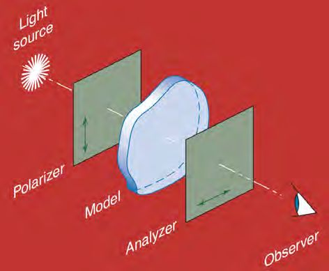
est largement utilisée dans des secteurs de technologie avancée comme l’aéronautique. Sa capacité à
simuler des structures complexes a conduit à élaborer des démarches hybrides calcul-photoélasticimétrie.
Plus qu’une complémentarité, il s’agit d’une véritable intégration de ces deux moyens prévisionnels.
Certains bureaux d’études, possédant de gros moyens de calculs, ont recours systématiquement à la
photoélasticité afin d’élaborer par exemple des hypothèses plausibles sur les conditions aux limites.
Cette technique est fondée sur le phénomène de biréfringence accidentelle ou effet photoélastique:
tout matériau solide transparent acquiert une biréfringence lorsqu’il est soumis à des sollicitations
mécaniques extérieures. L’ensemble des lois physiques décrivant ce phénomène constitue la photoélasticité.

                                                Montage expérimental
Le modèle consiste en une plaque photoélastique (un matériau photoélastique est un matériau dont
l’indice de réfraction dépend de la contrainte) 60 × 60mm, en polycarbonate ou en autres matériaux,
comportant une entaille d’environ 25mm de long, terminée par une amorce de fissure réalisée au moyen
d’une lame de rasoir. Un système vis-écrou permet d’appliquer une force provoquant l’ouverture de la
fissure (figure 2). Le banc de photoélasticité est composé d’une lampe à vapeur de mercure (utilisé pour
étudier les isoclines, figure 3), d’une lampe à vapeur de sodium (utilisé pour étudier les isochromes,
figure 3) et du modèle placé entre polariseurs croisés et lentilles (figure 2).

Figure 2: (gauche) Montage expérimental. (droit) Une plaque photoélastique avec le élément de contrainte au voisinage de la pointe
de fissure. (source: Experimental Stress Analysis, James W. Phillips).

              Figure 3: Une lampe à vapeur de mercure et une lampe à vapeur de sodium (source: google images).

                                                    Photoelastometry
In a photoelastic material the stress in some region of material influences the propagation of light
through that region. In particular, there is a birefringence effect: light polarized along the axis of
maximal principle stress, and the light polarized orhogonally (i.e., along axis of minimal principle
stress) are delayed in their propagation by different amounts. Based on Maxwell’s equations for
birefringence, the angular phase difference accumulated between the two orthogonal light waves is
                                                                      σ1 − σ2
                                                      ∆ = 2πhc                ,
                                                                         λ

                                                                  2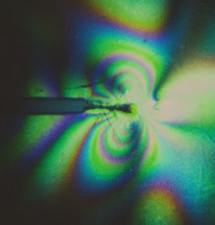
where σ1,2 are the two principal stresses (which are for us determined by the crack), the λ is the
wavelength of light (which is set by the lamp used), while the two parameters intrinsic to the chosen
piece of material are h, its thickness, and c, the relative stress-optic coefficient, which is independent
of λ.
    In our setup with an orthogonal polarizer and analyzer which sandwich the material (figure 2),
given the phase shift between two orthogonal components of light, it is straightforward to find the
intensity of observed light:
                                                             2
                                                             ∆
                                        I = a2 sin(2α)2 sin        ,
                                                              2
where α is the angle between the axis of maximal principal stress (σ1 ) and the axis of the analyzer,
the ∆ is the phase shift described above, and a is the amplitude of light leaving the polarizer.
    The application of photoelastometry in this TP is to extract information about the crack-induced
stress in the material, namely the principle stresses σ1,2 and the orientation of their axes at various
positions in the material, from observing the light intensity as you rotate the polarizer-analyzer pair
with respect to the material. The light intensity you will observe has two main features, isoclines
and isochromes, that will enable you to extract, respectively, the principle axes and the principal
stresses.

                                                             Isoclines
To start with, you will study the evolution of the isoclines emanating from the crack tip. Each point in
the material M (r, θ) is defined using polar coordinates r and θ with respect to the coordinate system
of the crack (figure 4). The θ is taken positive in the counterclockwise direction and ranges from −π
to π as you circle from just below the crack to just above it.

                                                                                        Isocline
                                                      Isocline

                                                                                                  Tangente

                                                                 crack

                                                                          Isocline
Figure 4: (left) γ is the angle the polarizer axis P1 makes with the x − axis measured in the clockwise direction. (right) θ is the
angle between the x − axis and the ”tangent” passing through the isocline measured in the counterclockwise direction. θP is the
angle between the isocline and the closest polarizer axis Pi measured in the counterclockwise direction. By definition θp cannot be
larger than 90o

     Isoclines are lines at which light completely vanishes, I = 0, no matter the color of light. They are
therefore given by the condition sin(2α)2 = 0, which is equivalent to α = m π2 , where m = 0, ±1, ±2, . . ..
In other words, at each point in the material M (r, θ) where the isocline is located, the local principle
stress axes are aligned with the axes defined by the polarizer and analyzer (figure 4).
     We first define the angle γ as the angle between one direction P1 on the polarizer axis and the
x-axis of the crack (figure 4). You will change this angle in the range 0 to 2π by rotating the po-
larizer dial (the analyzer should always remain perpendicular to the polarizer). In an infinitely large
photoelastic plate the isoclines would be straight lines, so you will approximate each isocline with a
”tangent” (like in figure 4), and you will assume that the isocline passes through all points M (r, θ),
i.e., through all r along the tangent with a certain value of θ. For any point M (θ) on an isocline you

                                                                    3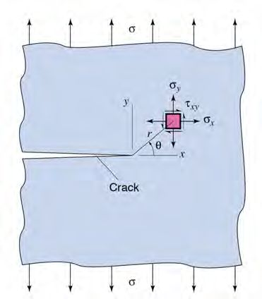
will record the two angles θ and γ (as explained we take this independent of r). According to the
photoelastometry model of isoclines, we can only deduce that the principle stress axes coincide with
the cross defined by P1,2,3,4 in figure 4. Knowing which of the arms of the cross is the P1 (tracked
by γ ∈ [0, 2π)) does not add information about principle stress axes. For this reason, and also for
usage in later part of the TP, we introduce a new angle variable θp which ranges only from 0 to π/2.
This range is enough to define the orientation of the cross and therefore the cross of principle stress
axes. The angle θp ∈ [0, π/2) for an isocline point M (θ) is defined as the counterclockwise rotation
angle needed to align the radial direction at M (θ) with a Pi axis closest to it (figure 4). In other
words, at a certain point M (θ) the angle θp measures the counterclockwise misalignment of the cross
defined by principle stress axes and the cross defined by radial coordinates. Automatically, you may
find the four directions Pi as the set Pn ≡ {γ + n π2 }, for n = 0, 1, 2, 3, and then choose the minimum
distance θp = minn {(−Pn − θ) mod 2π} (note: (1) the minus sign in front of Pn is due to opposite
sense of rotation of γ and θ; (2) the minimization should find the single distance that is in the range 0
to π/2). Collect data from all useful isoclines as you increase the polarizer angle γ in increments of 15o .

Your task is therefore to:
    • Deduce the dependence θp (θ) of the angle defining the principle stress axes on the position in
      material θ. The fitting function should be θp = mθ + θ0 . For all the measurements use ImageJ
      and for fitting use Python or Matlab.
NB:
(1) Due to effects not included in our modeling, you will may see either three or four isoclines.
(2) Isoclines in vicinity of the x-axis appear quite distorted, so avoid using them.

                                                     Isochromes
Isochromes are lines of vanishing light intensity, I = 0, obtained from the second condiction, namely,
      2
sin ∆
    2    = 0, which is equivalent to ∆ = 2πn, or
                                                           λ
                                                    σ1 − σ2 = n
                                                              ,                                            (1)
                                                           ch
where n = 0, ±1, ±2, . . .. As we consider a variation of color of light (λ), this condition will be satisfied
at varying points in the material, therefore non-monochromatic light produces a rainbow-like pattern
of colors. For this part of the exercise we therefore switch lamps and work with a monochromatic
source. Note that the isoclines are still present, but we instead focus on the isochromes which are
dark fringes identified by the red lobes in figure 5.

Figure 5: Isochromes - theoretical fringes for a KI (mode I) dominant field (source: Experimental Stress Analysis, James W.
Phillips).

  You will analyze the stress tensor in the material using the isochromes. In the simplest theoretical
model for the crack, the stress tensor has the form:
                                                         K
                                                  σij = √     fij (θ),                                                 (2)
                                                          2πr

                                                            4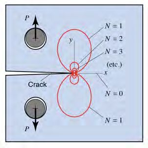
so that the magnitude of any stress, e.g., the principal stresses, depends on the distance from the crack
tip through a factor 1/r0.5 .

Analysis on line θ = const: finding f1 (r)
Following the line at θ = 90o which passes through the crack tip, find the intersections of this line
and the isochrome fringes. Measure each distance r(N ) from the crack point to an intersection, which
is labeled by the isochrome fringe order N . To obtain enough data points, you will have to load the
plate to see around 8 − 10 isochromes.

Your tasks are to:

   • Fit the datapoints (r, S) ≡ (r(N ), N ) to the curve S =      a
                                                                  rα   to find the exponent α.

   • Find the domain of validity of eq. 2.

   • Record the fit function S = f1 (r) you obtained.

NB:
(1) Be careful when loading the sample, there is a risk of propagating the crack, or even breaking the
plate.
(2) Follow attentively the order N of each isochrome as you load the plate.

Analysis on line r = const: finding f2 (θ)
Consider a circle of radius r centered on the crack tip (use ImageJ to draw the circle), and measure
the angular positions θ(N ) of successive isochromes N ; choose the radius r such that you stay within
the domain of validity of eq. 2 studied above.

Your tasks are:

   • In the measured datapoints (θ(N ), N ) if the θ(N ) is negative, also set its N to be negative (see
     figure 5).

   • Fit the datapoints (θ, S) ≡ (θ(N ), N ) by attempting simple trigonometric curves and record the
     best function S = f2 (θ). to find the exponent α. Record the fit function S = f1 (r) you obtained.
     Comment on the domain of validity of eq. 2.

   • Note that the free edges of the crack deform the stress field in the plate; in the ideal case, the
     field would be perfectly symmetric across the crack line. Consider the symmetry which the
     candidate functions for f2 should obey in this idealized case.

                                        Analysis of stress field
   • Using the results from this section, in view of eq. 1, write the principle stress difference σ1 − σ2
     as function of position M (r, θ) in plate, i.e., if σ1 − σ2 = J · f1 (r) · f2 (θ), what are the values of
     f1 (r) and f2 (θ).

   • By convention the factor J = 2√K2π . What is the physical dimension of the constant J? To
     which physical quantity does it relate?

                                                     5
Figure 6: Mohr’s circle for changing stress tensor under coordinate system rotations.
Mohr’s circle and the stress field in polar coordinates
Mohr’s circle enables us to simply and visually find the stress tensor in a rotated coordinate system
(figure 6). Note that the stress tensor is of second rank so its components get rotated in a more
complicated way than those of a vector. Nevertheless, Mohr’s circle correctly encodes all the rules.
You will use this tool together with a constraint equation on stresses to derive all components of stress
tensor in polar coordinates, σij (r, θ), i, j ∈ {r, θ}, just by using two quantities: the rotation angle
θp (θ) (derived from isoclines) and [σ1 − σ2 ](r, θ) (derived from isochromes).
A constraint equation which relates normal and tangential stresses at each point of a material in
the regime of linear elasticity and static equilibrium is:
∂σrr 1 ∂σrθ σrr − σθθ
+ + =0 (3)
∂r r ∂θ r
By definition of θp , at each point M (r, θ) we need to rotate the principal stress axes by an angle
ϕ ≡ −θp (θ) to align them to the radial coordinate axes (r, θ). In Mohr’s circle this always requires a
rotation by 2ϕ, see figure 6. Importantly, the photoelastometry gives us only the value of the difference
σ1 − σ2 , which is seen by Mohr’s circle to completely determine the maximal value of shear one can
observe by rotating the coordinates. From the known rotation ϕ, the shear component σrθ follows
straightforwardly.
Note that in the constraint equation you have: (1) the already found σrθ , (2) the σrr − σθθ which
depends only on the difference σ1 −σ2 (obvious in Mohr’s circle), and (3) the derivative of the unknown
field σrr . Integrate the partial differential equation and use the boundary condition that stress should
vanish at infinity.
Your tasks are:
• Deduce σrθ (r, θ) using Mohr’s circle (note, σθr ≡ σrθ ).
• Derive both σrr (r, θ) and σθθ (r, θ) by using the local constraint equation.
6Vous pouvez aussi lire