Utilisation de l'inférence Bayésienne pour la génération de ShakeMaps - RESIF
←
→
Transcription du contenu de la page
Si votre navigateur ne rend pas la page correctement, lisez s'il vous plaît le contenu de la page ci-dessous
Utilisation de l’inférence Bayésienne
       pour la génération de ShakeMaps

         2nd Workshop RESIF – Aléa sismique & Shakemaps
                Shakemap – Alternatives méthodologiques

Pierre Gehl – BRGM
Avec
John Douglas – University of Strathclyde
Dina D’Ayala – University College London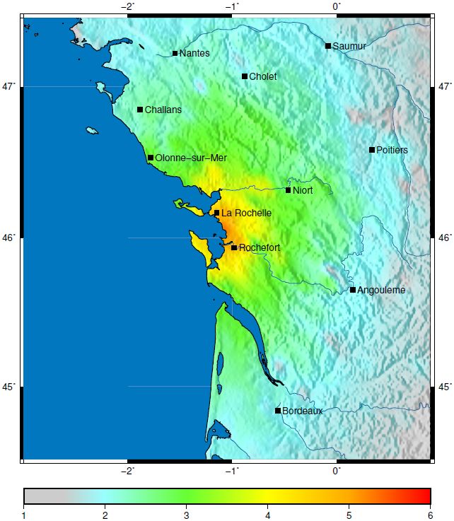
Principe de l’approche bayésienne
Réseau Bayésien                                                              Inférence bayésienne
                   Noeuds racines                        Distribution
    X1       X2    – Probabilité                         postérieure            X1         X2
                   marginale                             de X1

                   Noeuds descendants
    X4       X3    – Probabilité                                                X4         X3
                   conditionnelle

    X5                                                                          X5
                                                                                     Observation

>    Application à la génération d’une Shakemap
 Distribution a priori             Observations                         Distribution postérieure
Paramètres                   - Enregistrements par                     Mise à jour de la
probabilistes prédits        des stations                              distribution des paramètres
par une loi                  - Intensités ressenties                   par inférence
d’atténuation

                          2nd Workshop RESIF, Montpellier, 31 janvier 2018                          >2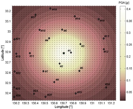
Principe de l’approche bayésienne
                    > Grille de 3x3 points
                    > 2 observations (e.g. PGA):
                                             >     Yobs1: 85% de l’estimation a priori
                                             >     Yobs2: 110% de l’estimation a priori

                                                                              Terme d’erreur
>   Réseau Bayésien correspondant:                                            inter-événement

                                                                                         Observations
        Paramètres sur
        la grille

    Corrélation spatiale
    des termes d’erreur
    intra-événement
                           2nd Workshop RESIF, Montpellier, 31 janvier 2018                        >3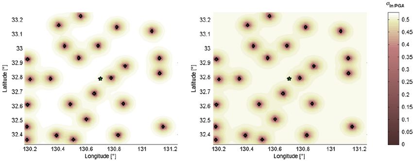
Principe de l’approche bayésienne

                                       Terme local (intra-
                                          événement)

                                                                                 Terme global
                                                                              (inter-événement)

     Terme local (intra-
        événement)

                           2nd Workshop RESIF, Montpellier, 31 janvier 2018                       >4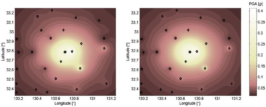
Traitement de plusieurs types d’observations

                                                                  MMI
   GMICE

                                                                  PGA

GMPE
                                                 Corrélation
                                                spatiale PGA

                                                Corrélation
                                               spatiale SA(T)

   GMPE

                                                                  SA(T)

               2nd Workshop RESIF, Montpellier, 31 janvier 2018           >5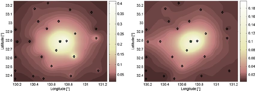
Validation – Séisme Mw 6.2 Kumamoto (2016)
                 PGA [g]                                          SA(1.0s) [g]

>   Grille de 48x48 points (100x100 km2)
>   26 stations sismiques
>   Estimation conjointe de PGA et SA(1.0s)
>   Résultats quasi-identiques à l’approche ShakeMap USGS
>   Traitement rigoureux de l’incertitude (équilibre entre les variabilités
    inter- et intra-événement)
                                           cf. Gehl et al. (2017) pour la validation analytique
                         2nd Workshop RESIF, Montpellier, 31 janvier 2018                    >6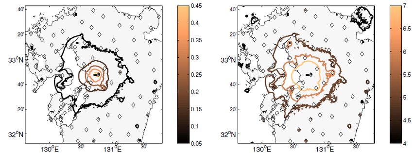
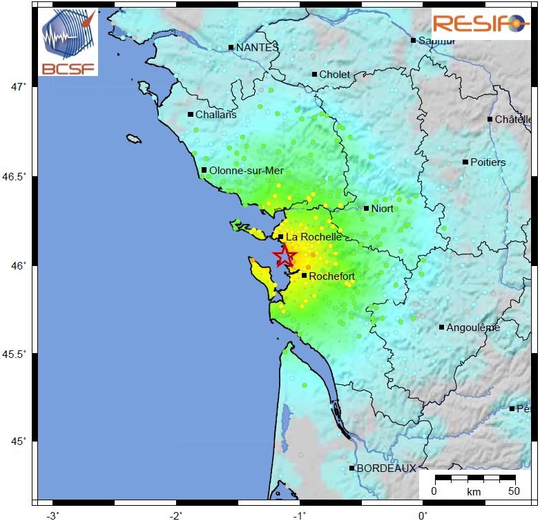
Test – Séisme ML 5.0 La Rochelle (2016)
> Peu d’observations intrumentales (2 stations)
> Nombreux témoignages (370 observations utilisées)
> ShakeMap en Intensité:

                    2nd Workshop RESIF, Montpellier, 31 janvier 2018   >7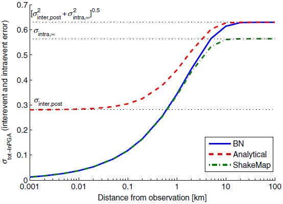
Test – Séisme ML 5.0 La Rochelle (2016)
> ShakeMap PGA:

   0.7% g (Franceséisme)
   1.4% g (Franceséisme)

                           2nd Workshop RESIF, Montpellier, 31 janvier 2018   >8
Test – Séisme ML 5.0 La Rochelle (2016)
> ShakeMap SA(1.0s)
2nd Workshop RESIF, Montpellier, 31 janvier 2018 >9Conclusions
> Intérêt de l’approche investiguée:
> Traitement rigoureux des sources d’incertitudes:
> Sigmas inter- et intra-événement
> Sigma des GMICEs
> Corrélation entre paramètres (e.g. PGA et SA)
> Possibilité d’obtenir des distributions conjointes de probabilités
> Performance accrue pour les séismes avec peu d’observations
> Défis à relever:
> Optimiser la rapidité d’exécution
> Influence des modèles de correlation spatiale
> Intégrer d’autres sources d’incertitudes (choix de GMPE,
magnitude, epicentre,…)
2nd Workshop RESIF, Montpellier, 31 janvier 2018 > 10Références
Bensi, M.T., Der Kiureghian, A. and Straub, D. (2011). A Bayesian Network methodology for infrastructure
seismic risk assessment and decision support. PEER Report 2011/02, Berkeley, California.
Gehl, P., Douglas, J., & D'Ayala, D. (2017). Inferring Earthquake Ground-Motion Fields with Bayesian
Networks. Bulletin of the Seismological Society of America, 107(6), 2792-2808.
Murphy, K. (2007). Bayes Net toolbox. Available from https://github.com/bayesnet/bnt.
2nd Workshop RESIF, Montpellier, 31 janvier 2018 > 11Spatially correlated ground motion fields
> Generic form for GMPEs: From Park et al. (2007)
Yi , j = f (θ i , j ) + ηi + ξ j
Inter-event error σinter Intra-event error σintra
- Common to all sites for - Correlated Gaussian field:
a given event
Where:
with
> Accounting for both cross-correlation and spatial correlation:
> Two IM types Y1 and Y2
> Cross-correlation coefficient ρ12
> 12General principles of Bayesian Networks
> BN = acyclic oriented graph è nodes (variables) and oriented edges
(statistical dependencies)
> Discrete or continuous Gaussian variables
BN structure BN inference
Root nodes Posterior
X1 X2 – Marginal distribution X1 X2
probability of X1
Child node
X4 X3 – Conditional X4 X3
probability
X5 X5
Evidence
> 13Bayesian inference from observations
> Use of continuous Gaussian BNs
> 14Demonstration on a synthetic example
> 3x3 grid (1 km grid step)
> Mw 5.5 EQ at coordinates [−3; 5]
> GMPE by Chiou & Youngs (2008)
> 2 single-IM observations:
> Yobs1: 15% smaller than GMPE estimate
> Yobs2: 10% larger than GMPE estimate
> Corresponding BN: Inter-event error
Observations
IMs at grid points
Intra-event
correlation structure
> 15Demonstration on a synthetic example
> Junction-tree algorithm:
> Updating of the probability distributions:
> 16Other shake-map methods
> The USGS SkakeMap algorithm (Worden & Wald, 2016):
> Removal of total bias from seismic records by adjusting
inter-event error term
> Interpolation between observations and bias-adjusted GMPE
estimates (weighted by distances from observations)
> Total ground-motion variability is computed from weighting of
intra-event error term with decay function
> Analytical solution (e.g. Stafford, 2012):
> Analytical resolution of a conditional multivariate normal
distribution
> 17Comparisons on the synthetic example
> Updated variables from the three methods:
> BN updating of mean values = analytical solution
> BN updating of inter-event error = analytical solution
> Total variability terms do not match
> 18Variability treatment
> Evolution of variability with distance from observation
limrà∞ σ2tot = σ2inter,post + σ2intra,post(∞)
limrà0 σ2tot = 0
> ShakeMap method: σ2inter,post set to zero
> Analytical solution: σ2inter,post and σ2intra,post are no longer
independent given observations
> 19Mw 6.2 Kumamoto foreshock on 14th Apr. 2016
Prior estimation > Metadata from USGS:
> Magnitude: Mw 6.2
> Depth: 9.0 km
> Longitude: 130.704°E
> Latitude: 32.788°N
> GMPE: Chiou and Youngs (2008, 2009)
> Total number of seismic stations: 194
> DYFI: 27 aggregated data points
> 100x100 km2 square grid
> 48x48 grid points
> 26 seismic stations considered
> 20Single-IM Bayesian inference
BN approach ShakeMap algorithm
PGA
shake-map
Uncertainty on
ln(PGA)
> 21Joint inference of cross-correlated IMs
PGA [g] SA(1.0s) [g]
> Ability to compute joint probabilities at a given site
> Helpful for the assessment of infrastructure systems affected by
multiple types of IM
> Seismic stations with missing data can still be used to constrain the
ground-motion field
> 22Accounting for macroseismic observations
PGA [g] MMI
> 200x200 km2 square grid
> 96x96 grid points
> 90 seismic stations considered + 14 macroseismic observations
è ~ 1 hour of processing time on a (slow) personal computer
> 23Vous pouvez aussi lire